Simple and unrestricted participation in SE listening tests neccessitates some post-screening procedure for rejecting evidently deviant grades submitted either by chance or intentionally or due to whatever reasons.
Some caution should be applied here as there is a danger of inappropriate shaping of collected data which can lead to invalid inference of their means. So there is a trade off between contamination of data with outlying grades and violation of data integrity through inappropriate shaping. Normally this kind of data shaping is not recommended for analysis of results of traditional listening tests (ITU-R BS.1116-1), but in case of SE testing there is a serious uncertanty about listeners' level of expertise, therefore some rejection mechanism is desirable.
In case of SE listening tests all submitted grades are annonymous because they belong to different people, who can't be identified reliably by recorded IP addresses. So the procedure has to analyze only grades but not subjects as recommended for traditional listening tests.
1. Data set
Below are descriptive statistics of 1626 test files and 13738 grades submitted to SE as of the end of 2009. Pairs of test files that differ in position of reference sample have been merged together. This data set is moderately contaminated with outliers as only severe ones were removed manually from time to time during the period of collection.
 | 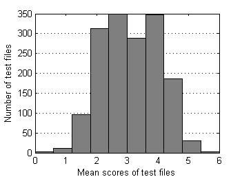 |
| Fig.1 Number of grades distribution over test files. | Fig.2 Mean score distribution over test files. |
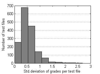 | 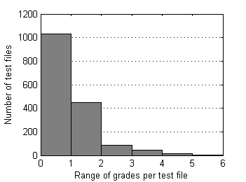 |
| Fig.3 Std. deviation of grades distribution over test files. | Fig.4 Range of grades distribution over test files. |
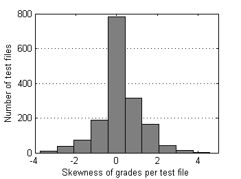 | 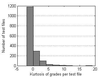 |
| Fig.5 Skewness of grades distribution over test files. | Fig.6 Kurtosis of grades distribution over test files. |
Note Grades “6” and “7” appear when listeners confuse reference and processed samples (“4” and “3” respectively); it was an idea to retain them for possible accounting in the future.
2. Rejection approaches
a) There are no methods to reliably separate submitted “6”s and “7”s into three groups:
- true grades when listeners prefer processed variant over reference
- inverted grades when listeners confused samples by mistake
- random grades
Actually this can be done with some probability but the whole system of post-screening will be more complicated, less transparent and more dependent on separation method. So it was decided to reject "6" and "7" grades completely.
b) Taking into account the nature of listening test experiment we could assume that submitted grades for a test file can't differ from each other too greatly. It's highly unlikely that a test file that has slightly annoying artifacts could be graded as imperceptible (“5”) or very annoying (“1”) the same time. In other words we could suppose the following rough relationship between “true” scores and possible grades for test files:
Table 1 Supposed relationship between "true" score of a test file and possible grades submitted for it. | "True" mean score | 1.0 | 1.5 | 2.0 | 2.5 | 3.0 | 3.5 | 4.0 | 4.5 | 5.0 |
| Possible grades | 1, 2 | 1, 2, 3 | 1, 2, 3 | 1, 2, 3, 4 | 2, 3, 4 | 2, 3, 4, 5 | 3, 4, 5 | 3, 4, 5 | 4, 5 |
In spite of speculative nature of that relationship we can safely assume that all grades are groupped around "true" mean within some radius. In the example above the radius is 1.5 and maximum range of grades is 3.0. Thus the second rejection rule could be formalized as:
M ± Rr, where
M - some parameter of central tendency of grades
Rr - radius of rejection which is supposed to be around 1.5 or higher; all grades beyond this radius are to be rejected.
c) All collected grades should be retained in DB and rejection should be applied on-the-fly each time new grade being received.
3. Testing rejection approaches on the data set
While rules (a) and (c) are pretty obvious, rule (b) is questionable:
- What parameter of central tendency should be used?
- Is rejection radius 1.5 adequate for the case? How it will affect mean scores of test files?
3.1. Parameter of central tendency
First we need to remove all “6”s and “7”s from our data set. All further operations will be applied to remaining grades only. Let this reduced data set be a control data set.
Arithmetic mean, trimmed mean and median are usual choices for estimator of central tendency. More sophisticated iterative M-estimators could lead to more efficient inference in the presence of outliers but adjusting of different parameters that control their performance turned out to be not trivial and needs more research. So at the moment we decided to limit our choice with more predictable traditional ones:
- Arithmetic mean
- Trimmed mean 20%
- Trimmed mean 30%
- Trimmed mean 40%
- Trimmed mean 50%
- Median
Let's assign constant value 1.5 to the rejection radius Rr at this stage. Then different estimators of location will cause slightly different rejection of grades. As a result we have six alternative data sets which can be analyzed and compared. Below are distributions of grades – in-liers and outliers - before and after rejection with different estimators.
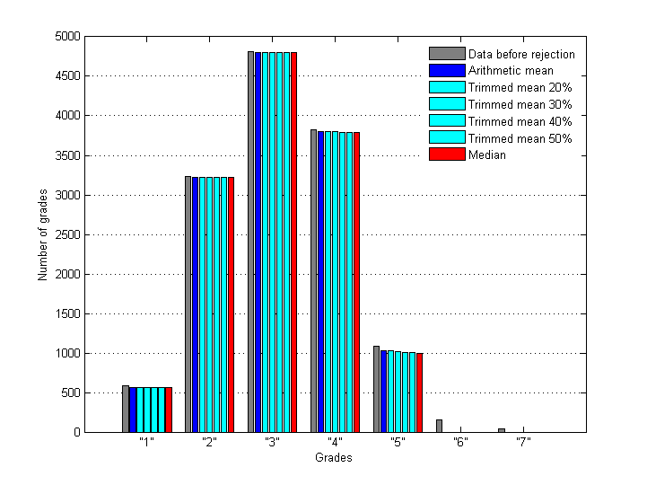
Fig.7 Distribution of inlying grades before and after applying of rejection rule with different estimators of central tendency (Rr = 1.5).
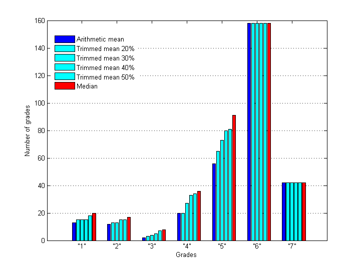
Fig.8 Distribution of outlying grades after applying of rejection rule with different estimators of central tendency (Rr = 1.5).
For sure there is some difference between estimators and now some test files in our six data sets have different mean scores comparing to the control data set. Let's estimate how many files were affected and how much they were affected in each of six cases. For the purpose we shall calculate three parameters for each data set:
- number of affected test files
- RMS and Max. deviations of mean scores of affected test files from corresponding mean scores in control set:
Table 2 Number of test files affected by different rejection rules (M±1.5) as well as RMS/Max deviations of mean scores for these affected files. | | Arithmetic mean | Trimmed mean 20% | Trimmed mean 30% | Trimmed mean 40% | Trimmed mean 50% | Median |
| Number of affected test files (files that changed their mean scores) | 95 | 103 | 113 | 125 | 131 | 144 |
| RMS deviation of the mean scores from control ones | 0.3362 | 0.3285 | 0.3251 | 0.3297 | 0.3389 | 0.3861 |
| Max deviation of the mean scores from control ones | 1.0 | 1.0 | 1.0 | 1.0 | 1.0 | 1.0 |
Use of median leads to higher number of rejected grades and consequently higher number of affected test files. Unfortunately there is no way to find out is it good or bad in our case, - whether these higher values of rejection are caused by median's higher robustness to outliers or by its lower efficiency as an estimator of central tendency (it can possess discrete values only - 1.0, 1.5, 2.0, …, 5.0). But if we separate all test files into groups according to number of grades per test file and compute those three parameters for each group, then we'll see the following regularity:
Table 3 Number of test files affected by different rejection rules (M±1.5) as well as RMS/Max deviations of mean scores for these affected files calculated for different groups of files; each group contains test files with equal number of collected grades. | Number
of grades
per file | Number
of files | Arithmetic
mean | Trimmed
mean 20% | Trimmed
mean 30% | Trimmed
mean 40% | Trimmed
mean 50% | Median |
| 3 | 133 | 3
0.8924
1.0000 | 3
0.8924
1.0000 | 3
0.8924
1.0000 | 3
0.8924
1.0000 | 3
0.8924
1.0000 | 14
0.7210
1.0000 |
| 4 | 186 | 6
0.7312
0.8333 | 6
0.7312
0.8333 | 6
0.7312
0.8333 | 6
0.7312
0.8333 | 11
0.6366
0.8333 | 11
0.6366
0.8333 |
| 5 | 166 | 4
0.4131
0.4500 | 4
0.4131
0.4500 | 4
0.4131
0.4500 | 12
0.3722
0.4500 | 12
0.3722
0.4500 | 13
0.4209
0.8000 |
| 6 | 167 | 7
0.3842
0.4667 | 7
0.3842
0.4667 | 7
0.3842
0.4667 | 9
0.3672
0.4667 | 9
0.3672
0.4667 | 8
0.3712
0.4667 |
| 7 | 104 | 4
0.3179
0.3810 | 4
0.3179
0.3810 | 6
0.3623
0.5714 | 6
0.3623
0.5714 | 6
0.3623
0.5714 | 8
0.4726
0.8571 |
| 8 | 100 | 8
0.2892
0.3750 | 8
0.2892
0.3750 | 8
0.2892
0.3750 | 8
0.2892
0.3750 | 9
0.3125
0.4583 | 9
0.3125
0.4583 |
| 9 | 90 | 9
0.2153
0.2500 | 9
0.2153
0.2500 | 14
0.2036
0.2500 | 14
0.2036
0.2500 | 14
0.2036
0.2500 | 14
0.2036
0.2500 |
| 10 | 84 | 6
0.2102
0.2444 | 7
0.2045
0.2444 | 7
0.2045
0.2444 | 8
0.2279
0.3500 | 8
0.2279
0.3500 | 8
0.2279
0.3500 |
| 11 | 102 | 13
0.2374
0.5253 | 13
0.2374
0.5253 | 13
0.2374
0.5253 | 13
0.2782
0.5455 | 13
0.2782
0.5455 | 13
0.2782
0.5455 |
| 12 | 70 | 2
0.3883
0.5278 | 2
0.3883
0.5278 | 2
0.3883
0.5278 | 3
0.3613
0.5278 | 3
0.3613 0.5278 | 3
0.3613 0.5278 |
| 13 | 84 | 10
0.1708
0.2937 | 13
0.2093
0.4385 | 13
0.2093
0.4385 | 13
0.2093
0.4385 | 13
0.2093 0.4385 | 13
0.2093 0.4385 |
| 14 | 50 | 3
0.1563
0.1703 | 3
0.1563
0.1703 | 6
0.2014
0.2381 | 6
0.2014
0.2381 | 6
0.2014 0.2381 | 6
0.2014 0.2381 |
| 15 | 50 | 3
0.1327
0.1476 | 4
0.1263
0.1476 | 4
0.1263
0.1476 | 4
0.1263
0.1476 | 4
0.1263 0.1476 | 4
0.1263 0.1476 |
| 16 | 40 | 1
0.1042
0.1042 | 2
0.1021
0.1042 | 2
0.1021
0.1042 | 2
0.1021
0.1042 | 2
0.1021 0.1042 | 2
0.1021 0.1042 |
| 17 | 27 | 5
0.1177
0.1471 | 5
0.1177
0.1471 | 5
0.1888
0.3613 | 5
0.1888
0.3613 | 5
0.1888 0.3613 | 5
0.1888 0.3613 |
| 18 | 15 | 3
0.0804
0.1013 | 3
0.0804
0.1013 | 3
0.0804
0.1013 | 3
0.0804
0.1013 | 3
0.0804 0.1013 | 3
0.0804 0.1013 |
| 19 | 12 | 2
0.1611
0.1920 | 3
0.1653
0.1920 | 3
0.1653
0.1920 | 3
0.1653
0.1920 | 3
0.1653 0.1920 | 3
0.1653
0.1920 |
| 20 | 9 | 2
0.1443
0.1833 | 2
0.1443
0.1833 | 2
0.1443
0.1833 | 2
0.1443 0.1833 | 2
0.1443
0.1833 | 2
0.1443
0.1833 |
For convenience numbers of affected test files from Table 3 are also presented on Fig.9.
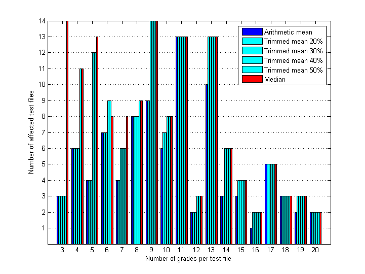
Fig.9 Number of test files affected by different rejection rules (M±1.5) and calculated for different groups of files; each group contains test files with equal number of collected grades.
With increase of number of grades per test file the difference between the estimators decreases. For small number of grades median results in higher rates of rejection. Starting from 13-14 grades all trimmed means and median result in rejection of the same grades (number of grades and RMS/Max deviations are the same). Starting from 18-19 grades all estimators operate equally.
Considering that:
- median is the most robust to outliers among all other estimators of central tendency
- median is better estimator of central tendency in case of deviations from normality of sample data and in case of small size of sample data
- gathering of 13-15 grades per test file is a common practice for listening tests and is not a problem for SE ones
it is preferable to use median as an estimator of central tendency for rejection of outlying grades in SE listening tests. For eliminating potential problems with low efficiency of median as an estimator of location the number of grades per test file should be around 15 or more.
3.2. Radius of rejection
First let's look at grade's standard deviations and ranges for test files from our control set (without “6”s and “7”s).
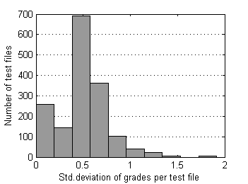
Fig.10 Distribution of std. deviation of grades over files
in control data set. | 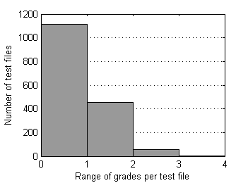
Fig.11 Distribution of range of grades over files
in control data set. |
And here is representation of these distributions by percentiles:
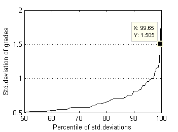
Fig.12 Std.deviation of grades distribution by percentiles. | 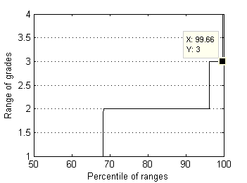
Fig.13 Range of grades distribution by percentiles. |
Almost all (99.7%) test files have grade's ranges below 3.0 and standard deviations below 1.5. Now supposed radius of rejection Rr=1.5 looks quite reasonable. In order to understand whether this rejection radius is acceptable or not, it's worth to research surrounding values as well. For larger perspective let's choose relatively wide interval [0.5, 2.5]. As median can possess discrete values only - 1.0, 1.5, 2.0, … , 5.0, we'll use in our research special case of Mean, which operates almost like Median but can possess arbitrary values. For simplisity let us intriduce the new estimator of location by example. For order statistic {X1, X2, X3, X4, X5} this special Mean – pfMean - is calculated by averaging auxiliary means M1...M7:
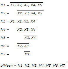
The parameter could be considered as mean, weighted towards median or average of trimmed means. It operates very similar to bootstrapped median but has less computational complexity and provides repetitive results for a given sample statistic. Also one can see other statistical hooks in calculating this parameter like Jackknifing, aggregating, sampling with/without replacement; the closest known statistical parameter with similar meaning is Trimean, but it has some restrictions on sample size. Considering all these as well as the method of the new parameter calculation a funny nickname “Pilfering Mean” well stuck to this estimator. We'll use it as a substitute to Median to test arbitrary values of rejection radius Rr.
For example relationship between rejection radius and number of affected test files from control set is on Fig.14:
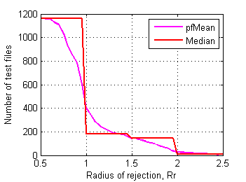
Fig.14 Number of affected test files in control data set depending on radius of rejection. |
Let's have a closer look at how characteristics of those affected files change as rejection radius decreases from 2.5 to 0.5. Fig.15 and Fig.16 show averages of std. deviations and ranges of grades in affected files depending on rejection radius.
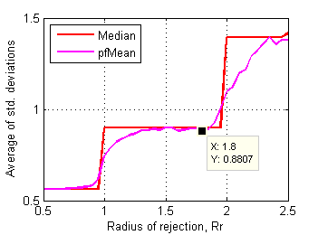
Fig.15 Average of std.deviations of affected test files
in control data set depending on radius of rejection. | 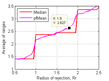
Fig.16 Average of ranges of affected test files
in control data set depending on radius of rejection. |
Steeper section above Rr~1.8 means that first cluster of affected files (~90 out of 1626) has substantially higher values of std. deviation and range. Further shortening of Rr below 1.8 affects another and bigger cluster of test files.
Skewness and kurtosis of affected files relate to rejection radius as follows:
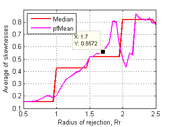
Fig.17 Average of skewnesses of affected test files
in control data set depending on radius of rejection. | 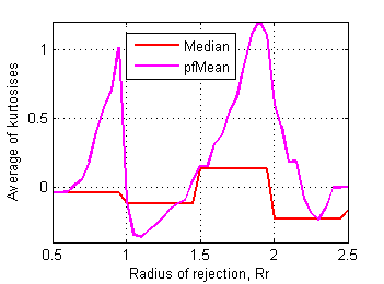
Fig.18 Average of kurtosises of affected test files
in control data set depending on radius of rejection. |
Border between clusters is less obvious here, may be Rr~1.7 on skewness plot has some sense. RMS deviation of mean scores of affected files from corresponding ones in control data set is more revealing (Fig.19):
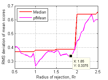
Fig.19 RMS deviation of mean scores of affected files from the ones in control data set depending on radius of rejection. |
Distinctive point Rr~1.85 clearly delimits first cluster of affected test files. These files dramatically change their mean scores after rejection of some grades. Considering all these plots another supposed value for rejection radius is 1.8.
Now we have two estimators of central tendency and two values for rejection radius. Total number of resulting rules of rejection is three:
- pfMean ± 1.8
- pfMean ± 1.5
- Median ± 1.5
Results of their application to our control data set are summerized in Table 4:
Table 4 Number of test files affected by different rejection rules as well as RMS/Max deviations of mean scores for these affected files. | | pfMean ± 1.8 | pfMean ± 1.5 | Median ± 1.5 |
| Number of affected test files (files that changed their mean scores) | 83 | 143 | 144 |
| RMS deviation of the mean scores from the ones in control set | 0.8807 | 0.8998 | 0.9002 |
| Max deviation of the mean scores from the ones in control set | 1.0 | 1.0 | 1.0 |
Total number of cases where at least one of the rejection rules triggers removal of grades is 145. It is not hard to compare them all "by hand". The complete list with comments is in Appendix 1. Manual peer reviewing of the cases reveals:
1) that performance of the rules “pfMean±1.5” and “Median±1.5” is almost identical, - only three cases out of 145 are different, in all of them “Median±1.5” performes better (see Appendix 2).
2) scores of appropriateness for each rule are in Table 5:
Table 5 Scores of appropriateness for each rule. | | pfMean±1.8 | pfMean±1.5 | Median±1.5 |
| Score of appropriateness relating to number of files affected by particular rule | 61/83
(73.5%) | 99/143
(69.2%) | 101/144
(70.1%) |
| Score of appropriateness relating to total number of affected files (145) | 82/145
(56.6%) | 99/145
(68.3%) | 102/145
(70.3%) |
Shortening the radius from 1.8 to 1.5 leads to higher number of affected files - 143 against 83, while percent of "better" cases stays the same - around 70%. Being calculated for all 145 cases scores of "pfMean±1.5" and "Median±1.5" are noticeably higher. It means that the value 1.5 could be safely used for rejection radius, it performs at least non the worse than 1.8 value.
Fig.20 shows results of contamination of reference data set with random grades (reference data set is the control data set cleaned with “Median ± 1.5” rule). Grades are added to random test files; number of added grades is proportional to number of existing grades in each test file; 50% contamination means that number of added and existing grades are equal. After each step of gradual contamination eight different rules of rejection are applied to contaminated data and RMS deviation of mean scores is calculated for each resulting (“cleaned”) data set.
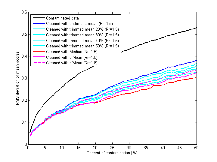
Fig.20 Results of contaminating reference data set with random grades and subsequent application of different rejection rules to contaminated data; for each case of "cleaning" the plot shows RMS deviation of mean scores of all (not only affected) test files.
Difference between contaminated and cleaned data is obvious. It is not surprising that median-based rule of rejection prevents changing of mean scores better than others, pfMean-based is the second. Increasing radius of rejection from 1.5 to 1.8 (dashed line) makes rejection mechanism slightly less efficient.
Thus, the recommended rejection rule for SE listening tests is Median ± 1.5 with min. 15 grades per test file (Median1.5/15).
As all collected grades are retained in SE data base it is recommended to repeat such research from time to time to reveal potential problems with rejection of grades. Being discovered they could be fixed increasing radius of rejection and using pfMean instead of median.
Appendix 1
List of all cases (145 out of 1626) where applying of at least one of rejection rules (pfMean ± 1.8, pfMean ± 1.5, Median ± 1.5) removes grades. In other words each test file in the list is affected by at least one of the rules.
Each case consists of four rows:
- original grades from control set
- grades after rejection with “pfMean ± 1.8” rule
- grades after rejection with “pfMean ± 1.5” rule
- grades after rejection with “Median ± 1.5” rule
For convenience the list is sorted by number of grades and has color marking:
- first row - original grades - are always black
- second row (pfMean ± 1.8) is black if unchanged (equal to first row) and magenta if some grades were rejected
- third row (pfMean ± 1.5) is magenta if unchanged (equal to second row) and orange if some grades were rejected
- fourth row (Median ± 1.5) is orange if unchanged (equal to third row) and red if some grades were rejected
Each case was peer reviewed for the appropriatness (A) of the rules application. If there is any kind of uncertanty about nesessity of particular rule application, such rule is marked with "0". Rule is marked with "1" only if there is high degry of confidence that application of particular rule is nesessary.
1 2 3 4 5 A
--------------
0 0 2 0 1
0 0 2 0 1 0
0 0 2 0 0 1
0 0 2 0 0 1
0 2 0 0 1
0 2 0 0 0 1
0 2 0 0 0 1
0 2 0 0 0 1
0 2 0 1 0
0 2 0 1 0 0
0 2 0 0 0 1
0 2 0 0 0 1
0 1 0 2 0
0 1 0 2 0 0
0 0 0 2 0 1
0 0 0 2 0 1
2 0 1 0 0
2 0 1 0 0 0
2 0 0 0 0 1
2 0 0 0 0 1
0 1 0 2 0
0 1 0 2 0 0
0 0 0 2 0 1
0 0 0 2 0 1
0 0 2 0 1
0 0 2 0 1 0
0 0 2 0 0 1
0 0 2 0 0 1
0 2 0 1 0
0 2 0 1 0 0
0 2 0 0 0 1
0 2 0 0 0 1
1 1 0 1 0
1 1 0 1 0 0
1 1 0 0 0 1
1 1 0 0 0 1
1 0 2 0 0
1 0 2 0 0 0
0 0 2 0 0 1
0 0 2 0 0 1
1 0 2 0 0
1 0 2 0 0 0
0 0 2 0 0 1
0 0 2 0 0 1
0 0 2 0 1
0 0 2 0 1 0
0 0 2 0 0 1
0 0 2 0 0 1
0 1 2 0 1
0 1 2 0 0 1
0 1 2 0 0 1
0 1 2 0 0 1
0 1 1 0 1
0 1 1 0 1 0
0 1 1 0 0 1
0 1 1 0 0 1
0 0 3 0 1
0 0 3 0 0 1
0 0 3 0 0 1
0 0 3 0 0 1
0 2 1 0 1
0 2 1 0 0 1
0 2 1 0 0 1
0 2 1 0 0 1
1 2 0 0 1
1 2 0 0 0 1
1 2 0 0 0 1
1 2 0 0 0 1
2 0 1 0 1
2 0 1 0 0 1
2 0 1 0 0 1
2 0 1 0 0 1
1 2 0 0 1
1 2 0 0 0 1
1 2 0 0 0 1
1 2 0 0 0 1
3 0 1 0 0
3 0 0 0 0 1
3 0 0 0 0 1
3 0 0 0 0 1
1 0 3 0 0
0 0 3 0 0 1
0 0 3 0 0 1
0 0 3 0 0 1
0 3 0 1 0
0 3 0 0 0 1
0 3 0 0 0 1
0 3 0 0 0 1
0 0 2 0 1
0 0 2 0 1 0
0 0 2 0 0 1
0 0 2 0 0 1
0 0 3 1 1
0 0 3 1 1 0
0 0 3 1 0 1
0 0 3 1 0 1
0 0 3 0 2
0 0 3 0 2 0
0 0 3 0 2 0
0 0 3 0 0 1
0 0 1 0 3
0 0 0 0 3 1
0 0 0 0 3 1
0 0 0 0 3 1
1 2 1 1 0
1 2 1 1 0 0
1 2 1 0 0 1
1 2 1 0 0 1
0 1 2 0 1
0 1 2 0 0 1
0 1 2 0 0 1
0 1 2 0 0 1
0 1 2 1 1
0 1 2 1 1 0
0 1 2 1 0 1
0 1 2 1 0 1
0 3 1 1 0
0 3 1 1 0 0
0 3 1 0 0 1
0 3 1 0 0 1
0 3 1 1 0
0 3 1 1 0 0
0 3 1 0 0 1
0 3 1 0 0 1
0 3 1 1 0
0 3 1 1 0 0
0 3 1 0 0 1
0 3 1 0 0 1
0 0 3 1 1
0 0 3 1 1 0
0 0 3 1 0 1
0 0 3 1 0 1
0 3 1 1 0
0 3 1 1 0 0
0 3 1 0 0 1
0 3 1 0 0 1
0 1 3 0 1
0 1 3 0 0 1
0 1 3 0 0 1
0 1 3 0 0 1
0 1 1 3 1
0 0 1 3 1 1
0 0 1 3 1 1
0 0 1 3 1 1
0 0 1 1 3
0 0 1 1 3 0
0 0 0 1 3 1
0 0 0 1 3 1
0 0 4 1 11
0 0 4 1 1 0
0 0 4 1 0 1
0 0 4 1 0 1
0 0 5 0 1
0 0 5 0 0 1
0 0 5 0 0 1
0 0 5 0 0 1
0 1 1 4 0
0 1 1 4 0 0
0 0 1 4 0 1
0 0 1 4 0 1
1 4 0 1 0
1 4 0 0 0 1
1 4 0 0 0 1
1 4 0 0 0 1
3 2 0 1 0
3 2 0 0 0 1
3 2 0 0 0 1
3 2 0 0 0 1
2 3 0 1 0
2 3 0 0 0 1
2 3 0 0 0 1
2 3 0 0 0 1
0 1 5 0 1
0 1 5 0 0 1
0 1 5 0 0 1
0 1 5 0 0 1
0 2 2 2 1
0 2 2 2 1 0
0 2 2 2 0 1
0 2 2 2 0 1
0 0 3 1 1
0 0 3 1 1 0
0 0 3 1 0 1
0 0 3 1 0 1
0 0 4 0 1
0 0 4 0 0 1
0 0 4 0 0 1
0 0 4 0 0 1
0 2 1 2 1
0 2 1 2 1 1
0 2 1 2 0 0
0 2 1 2 1 1
0 0 4 1 2
0 0 4 1 2 0
0 0 4 1 0 1
0 0 4 1 0 1
0 4 2 1 0
0 4 2 1 0 1
0 4 2 0 0 0
0 4 2 0 0 0
0 4 2 0 1
0 4 2 0 0 1
0 4 2 0 0 1
0 4 2 0 0 1
0 1 5 1 1
0 1 5 1 0 1
0 1 5 1 0 1
0 1 5 1 0 1
0 2 5 0 1
0 2 5 0 0 1
0 2 5 0 0 1
0 2 5 0 0 1
2 1 5 0 0
2 1 5 0 0 0
0 1 5 0 0 1
0 1 5 0 0 1
0 3 4 0 1
0 3 4 0 0 1
0 3 4 0 0 1
0 3 4 0 0 1
1 5 1 0 1
1 5 1 0 0 1
1 5 1 0 0 1
1 5 1 0 0 1
1 4 1 1 0
1 4 1 0 0 1
1 4 1 0 0 1
1 4 1 0 0 1
0 0 6 1 1
0 0 6 1 0 1
0 0 6 1 0 1
0 0 6 1 0 1
0 0 5 0 2
0 0 5 0 2 0
0 0 5 0 0 1
0 0 5 0 0 1
0 0 4 0 3
0 0 4 0 3 0
0 0 4 0 3 0
0 0 4 0 0 1
1 0 4 3 0
0 0 4 3 0 1
0 0 4 3 0 1
0 0 4 3 0 1
0 1 0 1 4
0 0 0 1 4 1
0 0 0 1 4 1
0 0 0 1 4 1
0 5 3 1 0
0 5 3 1 0 1
0 5 3 0 0 0
0 5 3 0 0 0
0 6 2 1 0
0 6 2 0 0 0
0 6 2 0 0 0
0 6 2 0 0 0
0 0 5 3 1
0 0 5 3 1 1
0 0 5 3 0 0
0 0 5 3 0 0
0 5 3 1 0
0 5 3 1 0 1
0 5 3 0 0 0
0 5 3 0 0 0
0 7 1 1 0
0 7 1 0 0 1
0 7 1 0 0 1
0 7 1 0 0 1
0 6 2 1 0
0 6 2 0 0 0
0 6 2 0 0 0
0 6 2 0 0 0
0 1 2 6 0
0 0 2 6 0 0
0 0 2 6 0 0
0 0 2 6 0 0
0 2 3 3 1
0 2 3 3 1 0
0 2 3 3 0 1
0 2 3 3 0 1
0 3 2 3 1
0 3 2 3 1 0
0 3 2 3 0 1
0 3 2 3 0 1
0 0 5 3 1
0 0 5 3 1 1
0 0 5 3 0 0
0 0 5 3 0 0
0 1 0 4 3
0 0 0 4 3 1
0 0 0 4 3 1
0 0 0 4 3 1
0 1 3 6 0
0 1 3 6 0 1
0 0 3 6 0 0
0 0 3 6 0 0
0 6 2 2 0
0 6 2 2 0 0
0 6 2 0 0 1
0 6 2 0 0 1
0 4 5 0 1
0 4 5 0 0 1
0 4 5 0 0 1
0 4 5 0 0 1
0 1 1 5 2
0 0 1 5 2 1
0 0 1 5 2 1
0 0 1 5 2 1
0 2 6 1 1
0 2 6 1 0 1
0 2 6 1 0 1
0 2 6 1 0 1
3 4 1 1 0
3 4 1 0 0 1
3 4 1 0 0 1
3 4 1 0 0 1
2 6 1 1 0
2 6 1 0 0 1
2 6 1 0 0 1
2 6 1 0 0 1
0 0 8 0 1
0 0 8 0 0 1
0 0 8 0 0 1
0 0 8 0 0 1
0 0 6 1 1
0 0 6 1 0 1
0 0 6 1 0 1
0 0 6 1 0 1
0 0 1 3 5
0 0 1 3 5 1
0 0 0 3 5 0
0 0 0 3 5 0
1 3 5 2 0
0 3 5 2 0 0
0 3 5 2 0 0
0 3 5 2 0 0
0 9 1 1 0
0 9 1 0 0 1
0 9 1 0 0 1
0 9 1 0 0 1
0 0 7 3 1
0 0 7 3 1 1
0 0 7 3 0 0
0 0 7 3 0 0
0 8 2 1 0
0 8 2 0 0 0
0 8 2 0 0 0
0 8 2 0 0 0
0 0 9 0 1
0 0 9 0 0 1
0 0 9 0 0 1
0 0 9 0 0 1
0 1 0 7 3
0 0 0 7 3 1
0 0 0 7 3 1
0 0 0 7 3 1
0 0 8 2 1
0 0 8 2 0 0
0 0 8 2 0 0
0 0 8 2 0 0
0 0 9 1 1
0 0 9 1 0 1
0 0 9 1 0 1
0 0 9 1 0 1
0 0 7 3 1
0 0 7 3 1 1
0 0 7 3 0 0
0 0 7 3 0 0
1 8 0 1 0
1 8 0 0 0 1
1 8 0 0 0 1
1 8 0 0 0 1
2 2 5 2 0
2 2 5 2 0 0
0 2 5 2 0 1
0 2 5 2 0 1
0 1 6 1 3
0 1 6 1 3 0
0 1 6 1 0 1
0 1 6 1 0 1
2 6 1 3 0
2 6 1 3 0 0
2 6 1 0 0 1
2 6 1 0 0 1
0 0 7 2 1
0 0 7 2 0 0
0 0 7 2 0 0
0 0 7 2 0 0
0 1 2 5 3
0 0 2 5 3 1
0 0 2 5 3 1
0 0 2 5 3 1
0 0 9 1 1
0 0 9 1 0 1
0 0 9 1 0 1
0 0 9 1 0 1
0 2 3 6 1
0 2 3 6 1 1
0 0 3 6 1 0
0 0 3 6 1 0
0 8 1 0 2
0 8 1 0 0 1
0 8 1 0 0 1
0 8 1 0 0 1
0 10 2 1 0
0 10 2 0 0 0
0 10 2 0 0 0
0 10 2 0 0 0
0 1 2 9 1
0 0 2 9 1 1
0 0 2 9 1 1
0 0 2 9 1 1
0 0 8 3 2
0 0 8 3 2 0
0 0 8 3 0 1
0 0 8 3 0 1
0 1 3 8 1
0 0 3 8 1 1
0 0 3 8 1 1
0 0 3 8 1 1
1 2 10 0 0
0 2 10 0 0 0
0 2 10 0 0 0
0 2 10 0 0 0
7 5 1 0 0
7 5 1 0 0 1
7 5 0 0 0 0
7 5 0 0 0 0
1 0 11 1 0
0 0 11 1 0 1
0 0 11 1 0 1
0 0 11 1 0 1
0 0 9 3 1
0 0 9 3 0 0
0 0 9 3 0 0
0 0 9 3 0 0
0 9 2 1 0
0 9 2 0 0 0
0 9 2 0 0 0
0 9 2 0 0 0
0 2 6 3 2
0 2 6 3 2 0
0 2 6 3 0 1
0 2 6 3 0 1
0 6 4 2 1
0 6 4 2 0 1
0 6 4 2 0 1
0 6 4 2 0 1
0 3 9 0 1
0 3 9 0 0 1
0 3 9 0 0 1
0 3 9 0 0 1
0 8 4 2 0
0 8 4 2 0 1
0 8 4 0 0 0
0 8 4 0 0 0
0 0 8 4 2
0 0 8 4 2 1
0 0 8 4 0 0
0 0 8 4 0 0
0 0 9 1 3
0 0 9 1 3 0
0 0 9 1 0 1
0 0 9 1 0 1
0 0 8 4 2
0 0 8 4 2 1
0 0 8 4 0 0
0 0 8 4 0 0
0 2 8 3 1
0 2 8 3 0 0
0 2 8 3 0 0
0 2 8 3 0 0
1 0 8 5 0
0 0 8 5 0 1
0 0 8 5 0 1
0 0 8 5 0 1
0 1 1 8 4
0 0 1 8 4 1
0 0 1 8 4 1
0 0 1 8 4 1
1 5 9 0 0
1 5 9 0 0 1
0 5 9 0 0 0
0 5 9 0 0 0
0 0 8 6 1
0 0 8 6 1 1
0 0 8 6 0 0
0 0 8 6 0 0
0 1 13 0 1
0 1 13 0 0 1
0 1 13 0 0 1
0 1 13 0 0 1
5 7 2 1 0
5 7 2 0 0 1
5 7 2 0 0 1
5 7 2 0 0 1
0 0 1 3 9
0 0 0 3 9 0
0 0 0 3 9 0
0 0 0 3 9 0
0 0 9 6 1
0 0 9 6 1 1
0 0 9 6 0 0
0 0 9 6 0 0
0 0 10 5 1
0 0 10 5 1 1
0 0 10 5 0 0
0 0 10 5 0 0
0 10 4 2 1
0 10 4 2 0 1
0 10 4 0 0 1
0 10 4 0 0 1
0 1 5 11 0
0 0 5 11 0 0
0 0 5 11 0 0
0 0 5 11 0 0
1 5 11 0 0
0 5 11 0 0 0
0 5 11 0 0 0
0 5 11 0 0 0
0 3 13 0 1
0 3 13 0 0 1
0 3 13 0 0 1
0 3 13 0 0 1
0 0 13 3 1
0 0 13 3 0 0
0 0 13 3 0 0
0 0 13 3 0 0
1 0 12 4 1
0 0 12 4 0 1
0 0 12 4 0 1
0 0 12 4 0 1
0 0 14 3 1
0 0 14 3 0 0
0 0 14 3 0 0
0 0 14 3 0 0
0 0 1 6 11
0 0 1 6 11 1
0 0 0 6 11 0
0 0 0 6 11 0
2 6 11 0 0
2 6 11 0 0 1
0 6 11 0 0 0
0 6 11 0 0 0
0 0 14 3 2
0 0 14 3 0 1
0 0 14 3 0 1
0 0 14 3 0 1
0 0 15 3 2
0 0 15 3 0 1
0 0 15 3 0 1
0 0 15 3 0 1
0 8 8 2 1
0 8 8 2 0 1
0 8 8 2 0 1
0 8 8 2 0 1
0 0 16 4 1
0 0 16 4 0 0
0 0 16 4 0 0
0 0 16 4 0 0
1 5 14 1 0
0 5 14 1 0 0
0 5 14 1 0 0
0 5 14 1 0 0
0 0 15 4 1
0 0 15 4 0 0
0 0 15 4 0 0
0 0 15 4 0 0
1 6 14 0 0
0 6 14 0 0 0
0 6 14 0 0 0
0 6 14 0 0 0
0 0 12 9 2
0 0 12 9 2 1
0 0 12 9 0 0
0 0 12 9 0 0
1 8 16 0 0
0 8 16 0 0 0
0 8 16 0 0 0
0 8 16 0 0 0
Appendix 2
Three cases from Appendix 1 where two rules - "pfMean±1.5" and "Median±1.5" - produce different output:
0 0 3 0 2
0 0 3 0 2 0
0 0 3 0 2 0
0 0 3 0 0 1
0 2 1 2 1
0 2 1 2 1 1
0 2 1 2 0 0
0 2 1 2 1 1
0 0 4 0 3
0 0 4 0 3 0
0 0 4 0 3 0
0 0 4 0 0 1