Abstract
Preliminary research at SoundExpert shows that there is high probability that relationship between waveform degradation of an audio material and its auditory perception does exist. This research is aimed to explore such relationship and its limitations. For the purpose several listening test cases (the more, the better) should be examined comparing levels of waveform degradation with subjective quality scores.
If such dependency is proved then reliable audio quality assessment will become easier and cheaper by means of:
- More productive listening tests. A listening test conducted for several contenders could provide quality scores for many more contenders with foreknown accuracy. Also results of an already finished listening test could be reused many times by adding new contenders afterwards and computing their quality scores analytically.
- Objective measurements with high correlation to subjective scores. Such measurements, based on statistical difference testing, can be translated into quality scores directly and will be valid for both analog and digital domains.
The research log below is updated live as the work goes on.
Case #1. Personal Listening Test of MP3/Opus/AAC at 96kbps by Kamedo2 (1 listener)
Draft. 2015 Nov 2. Research in progress ...
Results of this test were published on Hydrogen Audio forum (https://www.hydrogenaud.io/forums/index.php?showtopic=109716). The test was performed by one listener – Kamedo2 - using 74 sound samples.
Encoders:
LAME 3.99.5
Opus 1.1 with opus-tools-0.1.9, win32
NeroAACEnc 1.5.4.0
ffmpeg r.70351 with v7 patch applied
ffmpeg r.70351 with v9b patch applied
Settings:
lame --abr 98 -S in.wav out.mp3
opusenc --bitrate 91 in.wav out.opus
NeroAacEnc -q 0.333 -if in.wav -of out.mp4
ffmpeg70351_v7 -y -i in.wav -c:a aac -strict experimental -b:a 96k out.mp4
ffmpeg70351_v9b -y -i in.wav -c:a aac -strict experimental -b:a 96k out.mp4
Samples:
Total 74 samples.
40 samples from 2014 public listening test
25 samples from Kamedo2 corpus
9 samples from SoundExpert
Hardware:
Sony PSP-3000 + RP-HJE150.
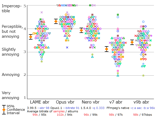 | Figure 1. Results of Kamedo2 listening test. |
So, we have the following mean scores of perceived sound quality:
opus   nero   lame   ffv9b   ffv7
4.31   3.93   3.65   3.42    3.13
Thanks to Kamedo2 all sources – sound samples and codec versions – are also available and can be used for objective/instrumental research.
Measurements of waveform degradation
Difference between original and processed by codecs waveforms will be measured in dB of Difference level (Df) with diffrogram program from here. We will use piece-wise Df measurements with time window of 400ms (impact of this parameter could be further researched). Such measurements produce multiple Df values (3568 in our case) which preserve valuable information about nature of waveform degradation.
Now we concatenate all 74 sound excerpts removing zero samples at the beginning and the end and applying 2.3ms cross-fade (100 samples) between excerpts. Thus we obtain a 1447s long (23:47) seamlessly mixed test vector containing sound material native to the Kamedo2 listening test. It is processed by all codecs with exact settings used in the listening test. As the decoded files have different sampling rates (32, 44.1, 48 kHz) they all are up-sampled to 96 kHz before Df calculations. Histograms of the resulting Df values for each codec are below:
| opus |  |
| nero |  |
| lame |  |
| ffv9b |  |
| ffv7 |  |
Figure 2. Histograms of Df values with native sound samples.
So, we have five medians of Df values showing level of waveform degradation for the codecs:
 opus       nero       lame       ffv9b      ffv7
-22.1849   -26.4295   -22.6954   -20.1345   -19.5650
Comparison of Df values with subjective scores
First, let's try linear best fit of those objective and subjective values:
df = [-22.1849 -26.4295 -22.6954 -20.1345 -19.5650];
 sq = [4.31 3.93 3.65 3.42 3.13]
 p = polyfit(df,sq,1);
 sqa = polyval(p,df)
 ((sqa-sq) ./ sq) * 100
 RMSE = sqrt(mean((sqa-sq).^2))
Table 1. Results of analytically computed quality scores using linear model and Df values as predictor variables with corresponding errors and total RMSError.
                        opus      nero     lame     ffv9b    ffv7    RMSEr

True Quality Score      4.31      3.93     3.65     3.42     3.13
Modeled Quality Score   3.69      4.12     3.74     3.48     3.42
Error                  -14.47%   +4.91%   +2.43%   +1.62%   +9.16%   0.32
While some errors are promising the whole picture is not encouraging – computed Opus score is too far (-14.5%) from its true value. The problem with aggregated Df values is that they do not take into account the type of waveform degradation, its nature. So we need some method to organize those Df values into groups with similar types of degradation. Required information about type of degradation is contained in full set of 3568 Df values. In fact, such Df sequence shows how different 400ms parts of audio signal were distorted during processing. Each Df sequence could be considered as a unique fingerprint of that particular processing. Thus, we can group/cluster those sequences according to their similarity to each other. Cluster analysis with correlation coefficient as a distance between sequences gives us the following result:
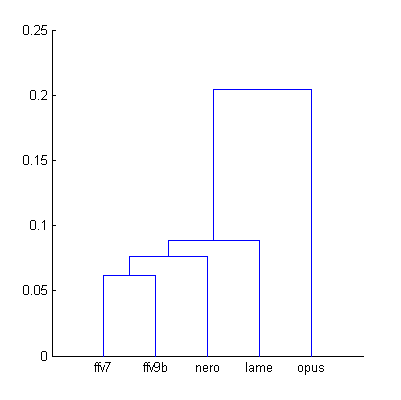 | Figure 3. Cluster analysis of Df sequences according to their similarity to each other. |
The dendrogram clearly shows that Opus Df sequence differs from the others. It should be excluded from our analysis. Remaining four Df sequences have similar fingerprints (less than 0.1 units of distance) and we can compute quality scores for them once again:
df = [-26.4295 -22.6954 -20.1345 -19.5650];
 sq = [3.93 3.65 3.42 3.13]
 p = polyfit(df,sq,1);
 sqa = polyval(p,df)
 ((sqa-sq) ./ sq) * 100
 RMSE = sqrt(mean((sqa-sq).^2))
Table 2. Results of analytically computed quality scores using linear model and Df values as predictor variables for the codecs excluding Opus.
                        opus     nero     lame     ffv9b    ffv7    RMSEr

True Quality Score      4.31     3.93     3.65     3.42     3.13
Modeled Quality Score            3.97     3.58     3.32     3.26
Error                           +0.99%   -1.83%   -2.97%   +4.14%   0.09
The fit is better now but it can be further improved. All SoundExpert experience with Difference level indicates that relationship between the latter and perceived sound quality is better modeled with second-order curve. Second-degree polinomial gives the following results:
df = [-26.4295 -22.6954 -20.1345 -19.5650];
 sq = [3.93 3.65 3.42 3.13]
 p = polyfit(df,sq,2);
 sqa = polyval(p,df)
 ((sqa-sq) ./ sq) * 100
 RMSE = sqrt(mean((sqa-sq).^2))
Table 3. Results of analytically computed quality scores using second-order model and Df values as predictors:
                        opus   nero     lame     ffv9b    ffv7    RMSEr

True Quality Score      4.31   3.93     3.65     3.42     3.13
Modeled Quality Score          3.92     3.68     3.31     3.21
Error                         -0.15%   +0.89%   -3.10%   +2.54%   0.07
And the fit can be improved even further using SoundExpert psychometric function which is in fact the same second-degree polinomial Ax2 + Bx + C but only curves where A>0 are used for modeling data. This function is used for calculation of “subjective” scores above 5-th grade in SE listening tests. In our case the function gives the following approximation to our true scores:
df = [-26.4295 -22.6954 -20.1345 -19.5650];
 sq = [3.93 3.65 3.42 3.13]
 sqa = sepsy(df, sq, df)
 er = ((sqa-sq) ./ sq) * 100
 RMSE = sqrt(mean((sqa-sq).^2))
Table 4. Results of analytically computed (modeled) quality scores using SoundExpert psychometric function (SE model) and Df values as predictors:
                        opus   nero     lame     ffv9b    ffv7    RMSEr

True Quality Score      4.31   3.93     3.65     3.42     3.13
Modeled Quality Score          3.93     3.67     3.38     3.22
Error                         -0.11%   +0.61%   -1.29%   +2.76%   0.05
It looks like this is the best fit we can get having the actual level of similarity for our Df sequences (error dependence on this similarity should be further researched).
Calculation of "missing" subjective scores
Now we are ready to perform an experiment aimed to show how good this methodology can predict results of the listening test. We will compute each of four quality scores (excluding Opus) using remaining three as inputs for our SE model. In other words, we will examine four cases of this listening test each time excluding one codec as if it did not participated in the test; subjective score of the “missing” codec will be computed analytically and can be compared with its true value.
% computing 'missing' Nero quality score
 DfN = -26.4295;
 SqN = 3.93;
 df = [-22.6954 -20.1345 -19.5650];
 sq = [3.65 3.42 3.13];
 sqaN = sepsy(df, sq, DfN)
 ErN = ((sqaN-SqN) ./ SqN) * 100
Table 5. Results of analytically computed quality scores for “missing” codecs:
                        opus   nero     lame     ffv9b    ffv7    RMSEr

True Quality Score      4.31   3.93     3.65     3.42     3.13
Missing Quality Score          3.85     3.70     3.32     3.36
Error                         -2.05%   +1.24%   -2.93%   +7.43%   0.13
Overall error increased, which is expected as the number of points for building our second-order model reduced from 4 to 3. But 7.5% error for ffv7 codec is a real fail. Nevertheless, computing of “missing” scores seems to be an appropriate procedure for testing our Df approach and for further research of factors affecting errors. One such factor could be sound material.
Impact of sound material
Why not to try sound material other than the one used by Kamedo2 in his listening test. At the end, those 74 sound excerpts are representative to some bigger population of music material. Also it would be helpful to have an idea how music material affects Df values and corresponding errors. For the purpose we'll use two variants - the whole album “The Dark Side of the Moon” and a random sequence of 450 small (4s) sound excerpts seamlessly concatenated into one half-an-hour post-modern masterpiece :-) For the both cases we will compute modeled and missing quality scores with corresponding errors.
The Dark Side of the Moon (42:53)
We will repeat the whole procedure of Df measurements with the album “The Dark Side of the Moon” as we did with the native sound excerpts: coding --> decoding --> upsampling --> Df values (6430 values by 400ms). Histograms are below:
| opus |  |
| nero |  |
| lame |  |
| ffv9b |  |
| ffv7 |  |
Figure 4. Histograms of Df values with “The Dark Side of the Moon” album.
We have five medians of Df values (dB) showing level of waveform degradation for the codecs with “The Dark Side of the Moon” album:
 opus       nero       lame       ffv9b      ffv7
-22.9455   -28.9768   -24.8911   -21.9785   -21.6071
Cluster analysis for these new Df sequences:
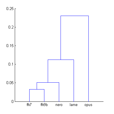 | Figure 5. Cluster analysis of Df sequences with “The Dark Side of the Moon” album. |
Comparing to native sound material we can say that Lame became less similar to aac family codecs but still around 0.1 units of distance; distance to Opus increased slightly. Anyway, for research purposes we will retain previous conditions for Df – SQ comparison - Opus is excluded from analysis.
Table 6. Modeled and missing quality scores with “The Dark Side of the Moon” album.
                        opus   nero     lame     ffv9b    ffv7    RMSEr

True Quality Score      4.31   3.93     3.65     3.42     3.13

Modeled Quality Score          3.92     3.68     3.36     3.26
Error                         -0.13%   +0.75%   -1.76%   +4.18%   0.07

Missing Quality Score          3.84     3.70     3.28     3.39
Error                         -2.36%   +1.51%   -4.11%   +8.25%   0.16
Using "The Dark Side of the Moon" album instead of native sound material increased the errors but not dramatically, which is a bit surprising and inspiring. Let's see what will happen with errors in case of using diverse collection of small excerpts (450 items, 4s each) smoothly mixed one after another.
The Random Mix (30:00)
The whole research procedure is exactly the same. Histograms are below:
| opus |  |
| nero |  |
| lame |  |
| ffv9b |  |
| ffv7 |  |
Figure 6. Histograms of Df values with The Random Mix
Five medians of Df values (dB) showing level of waveform degradation for the codecs with The Random Mix:
 opus       nero       lame       ffv9b      ffv7
-23.4859   -28.7681   -24.7532   -22.4382   -21.6660
Cluster analysis:
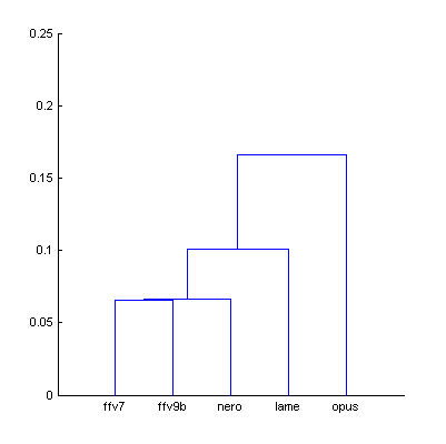 | Figure 7. Cluster analysis of Df sequences with The Random Mix. |
AAC family codecs look very similar now, Lame is still around 0.1 unit of distance from aac codecs, Opus still stands out from the others but to the less extent. Modeled and missing quality scores are below:
Table 7. Modeled and missing quality scores with The Random Mix
                        opus   nero     lame     ffv9b    ffv7    RMSEr

True Quality Score      4.31   3.93     3.65     3.42     3.13

Modeled Quality Score          3.93     3.66     3.40     3.19
Error                         -0.05%   +0.27%   -0.53%   +1.89%   0.03

Missing Quality Score          3.89     3.67     3.38     3.31
Error                         -1.03%   +0.56%   -1.19%   +5.86%   0.10
Results with arbitrary and highly diverse sound material are better than with the native one. This may happen thanks to unusually high number of sound excerpts (74) used in Kamedo2 listening test but this could also be a sign of more general regularity – the more audio material is used, the more level of its waveform degradation correlate with perceived audio quality. Shorter distances between Df sequences in cluster analysis with The Random Mix can be an indirect evidence of the latter. Experiment with substantially greater amount of audio material could be revealing in this sense. Also examination of other listening tests is necessary.
Adding new contenders to the listening test
As we have pretty good approximation to the true quality scores using SE model and The Random Mix (less than 2% error, Table 7), why not to add some new codec contenders to Kamedo2's listening test (hope he will not be against :). We will try three new codecs:
libfdk-aac 3.4.12; VBR mode 2; 96.03 kbit/s
fhgaac v03.02.16; VBR=3; 102.00 kbit/s
CoreAudioToolbox 7.10.5.0; AAC-LC Encoder; TVBR q45; 94.25 kbit/s
Random Mix was encoded/decoded with these new codecs and corresponding Df sequences were computed as usual:
Figure 8. Histograms of Df values of the new codecs with The Random Mix.
Three medians of Df values (dB) showing level of waveform degradation for the new codecs:
 fdk        fhg        tvbr
-27.6373   -29.8352   -23.4633
Cluster analysis:
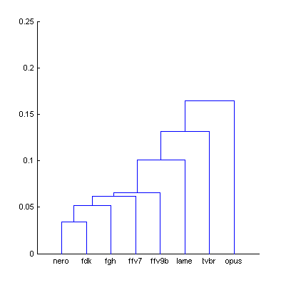 | Figure 9. Cluster analysis of Df sequences with The Random Mix and newly added codecs. |
Dendrogram clearly shows that aac codecs by Fraunhofer perfectly match our group (Nero and fdk are very very similar); tvbr aac codec from Apple is too far from them so we can't be sure that our model will work for it; we exclude it. Quality scores for remaining two codecs are computed using our second-order model.
Table 8. Modeled quality scores of native and post-test codecs (with The Random Mix).
                        opus     nero     lame     ffv9b    ffv7     fdk    fhg

True Quality Score      4.31     3.93     3.65     3.42     3.13

Modeled Quality Score            3.93     3.66     3.40     3.19     3.86    3.99
Error                           -0.05%   +0.27%   -0.53%   +1.89%

Bitrate with
The Random Mix, kbit/s  96.26    95.56    97.20    98.28    98.19    96.03   102.00
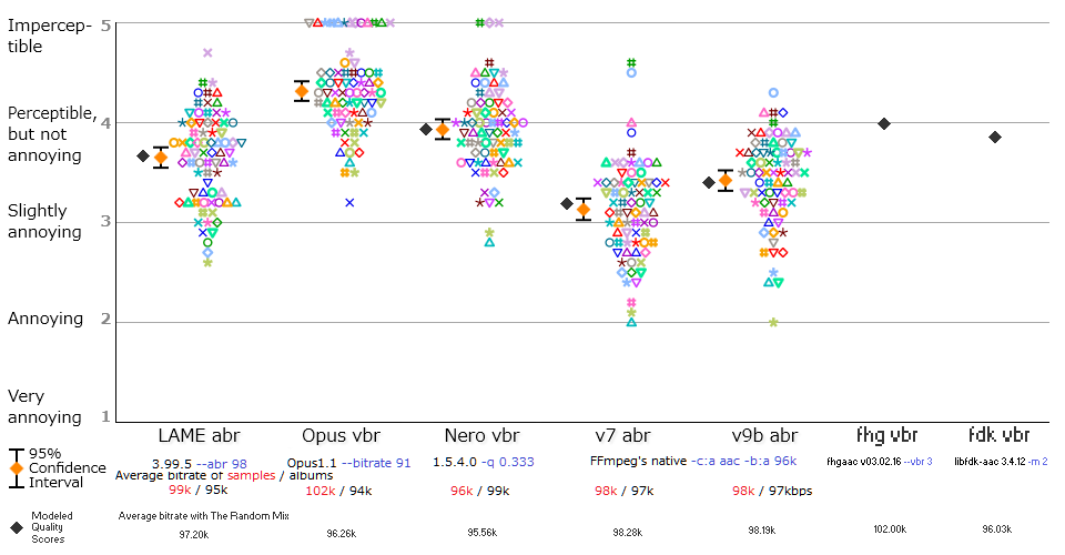
Figure 10. “Extended” Kamedo2 listening test with quality scores computed as the function of Difference levels (black diamonds).
Method of error estimation for such computed scores can be developed; there are two independent sources of the error – variance of true scores and non-similarity of Df sequences; bootstrapping may serve the purpose [more statistics and research needed].
Cluster analysis
2015 Nov 8
Finding similar Df sequences is important for building the model; this affects accuracy of predictions. We use cluster analysis for the purpose. On the first stage the algorithm finds distances between all Df sequences using (1 – r) as a measure of distance, where r is a correlation coefficient.
Table 9. Matrix of distances for Fig.3 as an example
         ffv7      ffv9      lame      nero      opus

ffv7         0    0.0621    0.0887    0.0796    0.2497
ffv9    0.0621         0    0.1192    0.0765    0.2507
lame    0.0887    0.1192         0    0.1133    0.2149
nero    0.0796    0.0765    0.1133         0    0.2042
opus    0.2497    0.2507    0.2149    0.2042         0
Codecs with short distances between each other can be used for building the model. For ease of choosing the suitable codecs the matrix of distances can be visualized with dendrogram. It shows the distances between elements and clusters of elements with U-shaped lines. For computing distances between clusters several methods can be used. In the Figures 3,5,7,9 dendrograms were computed using smallest distance between objects in two clusters. In our research another method which uses largest distance between objects in two clusters is more appropriate because it guarantees that max distance within group doesn't exceed some predefined value. Below are dendrograms from figures 3,5,7,9 computed using largest distance side by side with the old ones computed using smallest distance.
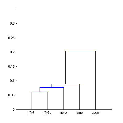 | 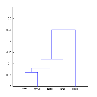 | Figure 3.1. Dendrogram from Fig.3 (native sound material), computed using smallest distance between objects in two clusters (a) and using largest distance (b). |
| a) | b) | |
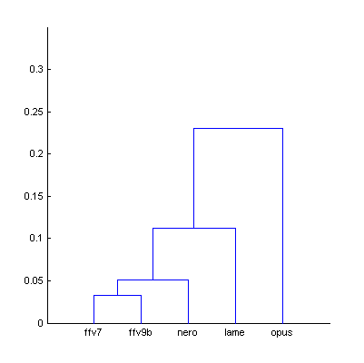 | 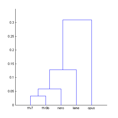 | Figure 5.1. Dendrogram from Fig.5 (The Dark Side of the Moon), computed using smallest distance between objects in two clusters (a) and using largest distance (b). |
| a) | b) | |
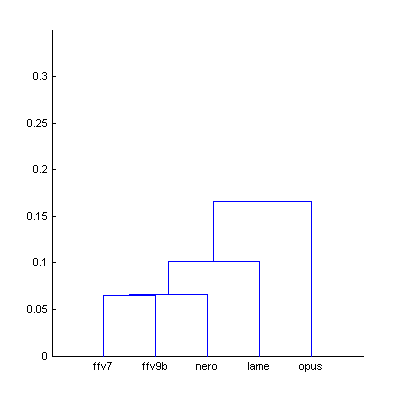 | 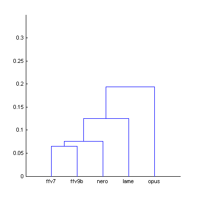 | Figure 7.1. Dendrogram from Fig.7 (The Random Mix), computed using smallest distance between objects in two clusters (a) and using largest distance (b). |
| a) | b) | |
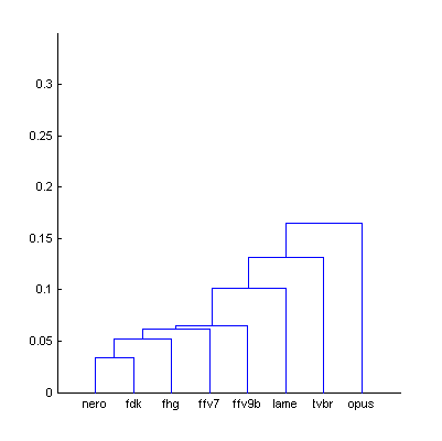 | 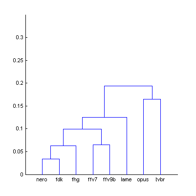 | Figure 9.1. Dendrogram from Fig.9 (The Random Mix), computed using smallest distance between objects in two clusters (a) and using largest distance (b). |
| a) | b) | |
Using largest distance between objects in two clusters allows better control consistency of distances within group, reliably removing outliers which decrease accuracy of the model. At this stage of research the distance of 0.1 units (cor.coeff = 0.9) looks sufficient [further research needed].
Increasing amount of sound material
For these three codecs – fhg, nero, tvbr – additional experiment was performed. Two dendrograms were computed: with The Random Mix (30:00, 450 excerpts) and with the extended random mix (120:00, 1800 excerpts).
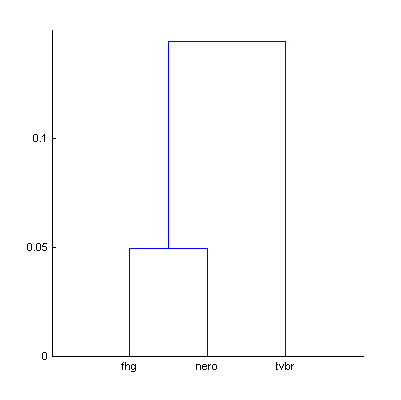 | 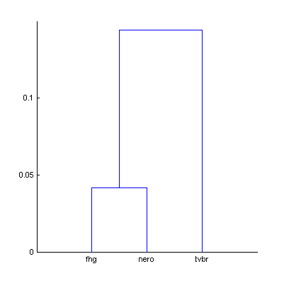 | Figure 11. Dendrograms of the three codecs with 450 (a) and 1800 (b) random sound excerpts. |
| (a) | (b) | |
Table 10. Df values and bitrates of the three codecs with 450 and 1800 sound excerpts extracted from different sound tracks of various genres.
               450 excerpts                  1800 excerpts
          Df,dB    Bitrate,kbit/s       Df,dB     Bitrate,kbit/s

fhg      -29.8352      102.00          -30.0331      101.63
nero     -28.7681       95.56          -29.0183       95.99
tvbr     -23.4633       94.85          -23.5182       95.29
Increased amount of random sound material didn't worsen cluster separation; vice versa – separation slightly increased. [Optimal amount of sound material should be defined].
... more of cluster analysis (the robust one)
2016 Jul 12
When Df sequences of the codecs were finally re-computed with higher precision (and different setting for time warping: 400ms instead of 30000ms used in previous low precision calculations), our cluster analysis showed different cluster separation of codecs.
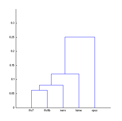 | 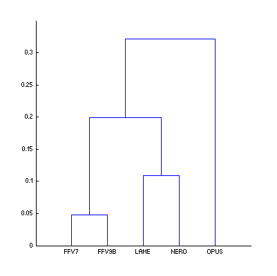 | Figure 12. Dendrograms of the codecs whose Df sequences were computed with low (a) and HIGH (b) precision. Our cluster analysis turned out to be too sensitive to the mode Df sequences were computed. |
| (a) | (b) |
Preliminary research revealed that Pearson correlation as a measure of similarity between Df sequences is not robust enough against small random variations in those sequences (low and HIGH precision Df sequences have almost similar distributions and medians; their histograms are in Fig.16). Another measure of similarity should be found for our research. As we are interested in similarity of shapes of Df sequences the required measure most probably will be based on correlation. Two robust versions of correlation coefficient - Spearman's rank correlation and the recent Distance correlation [G. J. Szekely; M. L. Rizzo; N. K. Bakirov (2007), "Measuring and Testing Independence by Correlation of Distances"] – showed most promising results (Fig.13) and will be examined below.
Figure 13. Dendrograms of the codecs computed using different measures of similarity: Pearson correlation (a), Spearman's rank correlation (b) and Distance correlation (c). Both the low and HIGH precision versions of Df sequences are shown together to better reveal the problem with Pearson correlation. The latter not only failed to separate correctly the clusters of codecs but also failed to find correctly the similarities between the low and HIGH versions of the codecs' Df sequences (ffv7 and ffv9b).
The figures clearly show that Spearman's rank correlation and Distance correlation perform much better and have close results. Let's find out if there is an advantage of one over another in our case. We already know for sure (and it was confirmed by previous cluster analyses) that Opus and AAC codecs belong to separate clusters. So we can estimate effectiveness of each measure of distance by computing average distance within AAC cluster (it must be minimal) and average distance between Opus and AAC codecs (it must be maximal). Results of such measurements (including Pearson correlation) are below.
Table 11. Matrices of normalized distances (Dmax = 1) between codecs (Native sound samples (74), low precision) computed using different measures of distance/similarity and corresponding WITHIN and BETWEEN measurements for Opus and AAC clusters.
| Native sound samples (74), low precision, D:correlation
ffv7 ffv9b lame nero opus
ffv7 0 0.2475 0.3536 0.3173 0.9957
ffv9b 0.2475 0 0.4753 0.3052 1.0000
lame 0.3536 0.4753 0 0.4520 0.8572
nero 0.3173 0.3052 0.4520 0 0.8142
opus 0.9957 1.0000 0.8572 0.8142 0 | Average distance Average distance
WITHIN aac cluster BETWEEN opus-aac
0.28997 0.93663 |
| Native sound samples (74), low precision, D:spearman
ffv7 ffv9b lame nero opus
ffv7 0 0.2323 0.5061 0.4111 0.9628
ffv9b 0.2323 0 0.4785 0.4414 1.0000
lame 0.5061 0.4785 0 0.4640 0.7919
nero 0.4111 0.4414 0.4640 0 0.8670
opus 0.9628 1.0000 0.7919 0.8670 0 | Average distance Average distance
WITHIN aac cluster BETWEEN opus-aac
0.36159 0.94327 |
| Native sound samples (74), low precision, D:distance correlation
ffv7 ffv9b lame nero opus
ffv7 0 0.2722 0.5601 0.4266 0.9852
ffv9b 0.2722 0 0.5321 0.4518 1.0000
lame 0.5601 0.5321 0 0.5146 0.8275
nero 0.4266 0.4518 0.5146 0 0.8563
opus 0.9852 1.0000 0.8275 0.8563 0 | Average distance Average distance
WITHIN aac cluster BETWEEN opus-aac
0.38354 0.94718 |
Table 12. Matrices of normalized distances (Dmax = 1) between codecs (Native sound samples (74), HIGH precision) computed using different measures of distance/similarity and corresponding WITHIN and BETWEEN measurements for Opus and AAC clusters.
| Native sound samples (74), HIGH precision, D:correlation
FFV7 FFV9B LAME NERO OPUS
FFV7 0 0.1488 0.5572 0.4454 1.0000
FFV9B 0.1488 0 0.6168 0.4500 0.9999
LAME 0.5572 0.6168 0 0.3373 0.6671
NERO 0.4454 0.4500 0.3373 0 0.6005
OPUS 1.0000 0.9999 0.6671 0.6005 0 | Average distance Average distance
WITHIN aac cluster BETWEEN opus-aac
0.34805 0.86682 |
| Native sound samples (74), HIGH precision, D:spearman
FFV7 FFV9B LAME NERO OPUS
FFV7 0 0.2455 0.5043 0.3493 0.9496
FFV9B 0.2455 0 0.4892 0.3883 1.0000
LAME 0.5043 0.4892 0 0.4014 0.7905
NERO 0.3493 0.3883 0.4014 0 0.8064
OPUS 0.9496 1.0000 0.7905 0.8064 0 | Average distance Average distance
WITHIN aac cluster BETWEEN opus-aac
0.32772 0.91868 |
| Native sound samples (74), HIGH precision, D:distance correlation
FFV7 FFV9B LAME NERO OPUS
FFV7 0 0.2763 0.5627 0.3799 0.9783
FFV9B 0.2763 0 0.5339 0.4054 1.0000
LAME 0.5627 0.5339 0 0.4589 0.8211
NERO 0.3799 0.4054 0.4589 0 0.7943
OPUS 0.9783 1.0000 0.8211 0.7943 0 | Average distance Average distance
WITHIN aac cluster BETWEEN opus-aac
0.35387 0.9242 |
Table 13. Matrices of normalized distances (Dmax = 1) between codecs (Random mix (450), low precision) computed using different measures of distance/similarity and corresponding WITHIN and BETWEEN measurements for Opus and AAC clusters.
| Random mix (450), low precision, D:correlation
ffv7 ffv9b lame nero opus
ffv7 0 0.3383 0.6134 0.3413 1.0000
ffv9b 0.3383 0 0.6497 0.3932 0.9571
lame 0.6134 0.6497 0 0.5230 0.9727
nero 0.3413 0.3932 0.5230 0 0.8574
opus 1.0000 0.9571 0.9727 0.8574 0 | Average distance Average distance
WITHIN aac cluster BETWEEN opus-aac
0.35761 0.93818 |
| Random mix (450), low precision, D:spearman
ffv7 ffv9b lame nero opus
ffv7 0 0.3484 0.6350 0.3521 0.9615
ffv9b 0.3484 0 0.6660 0.4232 1.0000
lame 0.6350 0.6660 0 0.5007 0.9118
nero 0.3521 0.4232 0.5007 0 0.8363
opus 0.9615 1.0000 0.9118 0.8363 0 | Average distance Average distance
WITHIN aac cluster BETWEEN opus-aac
0.37459 0.93261 |
| Random mix (450), low precision, D:distance correlation
ffv7 ffv9b lame nero opus
ffv7 0 0.3587 0.6884 0.3660 0.9944
ffv9b 0.3587 0 0.7094 0.4325 1.0000
lame 0.6884 0.7094 0 0.5574 0.9444
nero 0.3660 0.4325 0.5574 0 0.8413
opus 0.9944 1.0000 0.9444 0.8413 0 | Average distance Average distance
WITHIN aac cluster BETWEEN opus-aac
0.38576 0.94523 |
Table 14. Matrices of normalized distances (Dmax = 1) between codecs (Random mix (450), HIGH precision) computed using different measures of distance/similarity and corresponding WITHIN and BETWEEN measurements for Opus and AAC clusters.
| Random mix (450), HIGH precision, D:correlation
FFV7 FFV9B LAME NERO OPUS
FFV7 0 0.3522 0.6656 0.3142 0.9969
FFV9B 0.3522 0 0.6958 0.4095 0.9786
LAME 0.6656 0.6958 0 0.5914 1.0000
NERO 0.3142 0.4095 0.5914 0 0.8701
OPUS 0.9969 0.9786 1.0000 0.8701 0 | Average distance Average distance
WITHIN aac cluster BETWEEN opus-aac
0.35864 0.94854 |
| Random mix (450), HIGH precision, D:spearman
FFV7 FFV9B LAME NERO OPUS
FFV7 0 0.3341 0.6367 0.2843 0.9199
FFV9B 0.3341 0 0.6945 0.4151 1.0000
LAME 0.6367 0.6945 0 0.5340 0.9358
NERO 0.2843 0.4151 0.5340 0 0.8338
OPUS 0.9199 1.0000 0.9358 0.8338 0 | Average distance Average distance
WITHIN aac cluster BETWEEN opus-aac
0.34453 0.91792 |
| Random mix (450), HIGH precision, D:distance correlation
FFV7 FFV9B LAME NERO OPUS
FFV7 0 0.3462 0.7014 0.3130 0.9601
FFV9B 0.3462 0 0.7389 0.4260 1.0000
LAME 0.7014 0.7389 0 0.5959 0.9681
NERO 0.3130 0.4260 0.5959 0 0.8438
OPUS 0.9601 1.0000 0.9681 0.8438 0 | Average distance Average distance
WITHIN aac cluster BETWEEN opus-aac
0.36173 0.93463 |
From the tables:
- both Spearman's rank correlation and Distance correlation have close results;
- Spearman's rank correlation has slightly lower WITHIN values; this helps to better reveal the similarities within aac cluster.
- Distance correlation has slightly higher BETWEEN values; this helps to better reveal the distinctions between Opus and aac clusters;
- Pearson correlation has the best WITHIN-BETWEEN values in all cases except where it fails completely (Native sound samples (74), HIGH precision).
It looks like both Spearman and Distance correlations should be used in our audio research for better consistency of results.
And finally we should choose the right linkage method for building dendrograms, the one, which better visualizes distance information contained in distance matrices and thus gives correct clusterization of codecs. We will examine three well-known methods - single, complete and average linkages and the new one – E-clustering [Gabor J. Szekely; Maria L. Rizzo (2012), "Energy statistics: A class of statistics based on distances"]. It must be noted that the use of E-clustering is questionable in our case because the method is defined for Euclidean distances (metric spaces) only. In general case distances produced by correlation measurements belong to non-metric space. However, triangle inequality test applied to our distance matrices revealed that all of them comply with the test. The exceptions are distance matrices for the cases of the low/HIGH precision Df sequences being analyzed together (Fig.13). In these cases triangle inequality holds for ~98% of all possible distance triangles between 10 codecs. Perhaps, if triangle inequality holds for 100%, then the distances could be treated as Euclidean [further research needed]. So, we will use E-clustering method in our case with caution, as an experiment.
In order to estimate effectiveness of these four methods of linkage we will use cophenetic correlation coefficient, which measures how good a dendrogram represent the distances from distance matrix. The higher the value (Cph <= 1) the better dendrogram reflects similarity/dissimilarity between codecs.
Df sequences for native sound samples (74) and random mix (450), both computed with low and HIGH precision, will be used for our linkage test. Three such dendrograms for complete linkage and three measures of distance (Pearson correlation, Spearman correlation, Distance correlation) were already shown in Fig.13. Now we'll plot the whole set of dendrograms for these three measures of distance and the four linkage methods - single, complete, average, E-clustering. For each dendrogram the cophenetic correlation coefficients will be computed. Resulting plots are below.
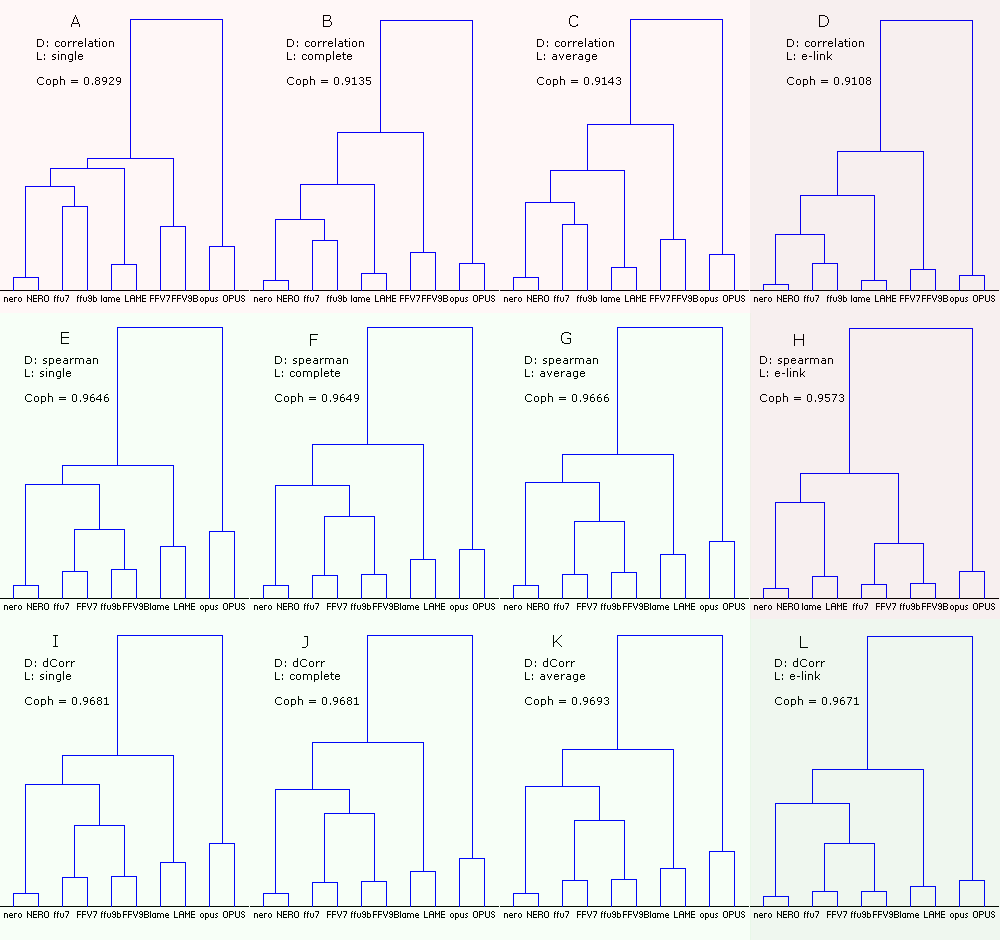
Figure 14. Dendrograms of the codecs with the native sound samples (74). Df sequences for the codecs were computed twice - with low and the HIGH precision (ten sequences in total). The dendrograms were plotted using three measures of distance and four linkage methods.
From the figure:
- the right column (DHL) corresponding to E-clustering is a Grey area as the use of this method is questionable due to non-metric nature of our distances/similarities between Df sequences (~98% compliance with triangle inequality test);
- Pearson correlation as a measure of distance gives wrong clustering of codecs (ABCD); combination of Spearman correlation and E-clustering (H) also fails; all wrong dendrograms have lower cophenetic correlation and marked reddish;
- combination of Spearman/Distance correlations and single/complete/average linkages (EFGIJK) gives consistent and predictable clustering; they are greenish;
- for all linkage methods Distance correlation has slightly higher cophenetic correlation (IJKL);
- for all measures of distance average linkage has slightly higher cophenetic correlation (CGK);
- combination of Distance correlation and E-clustering (L) gives the best separation of the codecs; also this combination is outstanding in determination of similarities between the low and HIGH versions of the same codecs (lowest linkages between the versions); also for all measures of distance E-clustering (DHL) gives the lowest linkages between the low and HIGH versions of the same codecs.
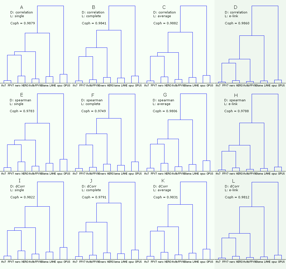
Figure 15. Dendrograms of the codecs with the random mix (450). Df sequences for the codecs were computed twice - with low and HIGH precision (ten sequences in total). The dendrograms were plotted using three measures of distance and four linkage methods.
From the figure:
- the right column (DHL) corresponding to E-clustering is a Grey area as the use of this method is questionable due to non-metric nature of our distances/similarities between Df sequences (~98% compliance with triangle inequality test);
- in case of the random mix (450) all combinations of distance measures and linkages give similar results (all greenish); there are some differences within aac cluster in case of complete linkage (BFJ) but these dendrograms have slightly lower cophenetic correlation;
- for all linkage methods Pearson correlation has slightly higher cophenetic correlation (ABCD); Distance correlation is the second;
- for all measures of distance average linkage has slightly higher cophenetic correlation (CGK);
- as in previous case with the native sound samples (74) combination of Distance correlation and E-clustering (L) gives the best separation of the codecs; also this combination is outstanding in determination of similarities between the low and HIGH versions of the same codecs (lowest linkages between the versions); also for all measures of distance E-clustering (DHL) gives the lowest linkages between the low and HIGH versions of the same codecs.
Conclusion: for consistent and reliable cluster analysis (which plays important role in our audio research) it is advisable to use at least two different ways of clusterization; one – more classical – Spearman's rank correlation + average linkage, which is simple and easy to interpret; another – more sophisticated – Distance correlation + E-clustering, which is surprisingly powerful but has questionable correctness in our case (results of triangle inequality test must be supplied).
The research method
2016 Jul 29
Finally the methods and research instruments have been pretty defined.
In each listening test case we will compare objective measurements with subjective scores using two types of audio material:
- native sound samples that were used during listening test - Native Audio
- one and the same random mix consisting of 450 short (4sec) sound samples of various artists - The Random Mix, 30min
Objective measurements will be represented by sequences of Df values showing degradation of initial waveform piece-wise with 0.4sec window (and 0.4sec frame for time warping). Histograms of the sequences with medians and percentiles will be provided.
Comparison of Df sequences with each other will be performed by means of cluster analysis using two measures of distance:
- Spearman's rank correlation
- Distance correlation
and two linkage methods:
- average linking for Spearman's rank correlation
- energy linking for Distance correlation (results of triangle inequality test will be provided)
Upon the results of the cluster analysis a group of codecs with similar nature of waveform degradation will be chosen and be used for further research. For such codec group average distance within group and max distance will be provided (for both distance measures).
For chosen group of codecs the simple regression analysis will be performed using quadratic curve fitting between medians of Df sequences and corresponding subjective scores. Differences (residuals) between true subjective scores and the ones predicted by the model will be provided (as in Table 4).
In accordance with this methodology the research case with kamedo2 listening test can be summarized as follows.
1. True subjective scores.
Table 15. Subjective quality scores from the listening test.
opus   nero   lame   ffv9b   ffv7
4.31   3.93   3.65   3.42    3.13
2. Df measurements.
| OPUS |
 |  |
| NERO |
 |  |
| LAME |
 |  |
| FFV9B |
 |  |
| FFV7 |
 |  |
(a)
| (b)
|
Figure 16. Df measurements with native audio material (a) and the random mix (b).
3. Cluster analysis
Table 16. Distances between codecs with native audio material (left) and the random mix (right) and two measures of distance: Spearman's rank correlation (top) and Distance correlation (bottom). All distances comply with triangle inequality test.
| FFV7 FFV9B LAME NERO OPUS
FFV7 000000 0.0465 0.0954 0.0661 0.1797
FFV9B 0.0465 000000 0.0926 0.0735 0.1892
LAME 0.0954 0.0926 000000 0.0760 0.1496
NERO 0.0661 0.0735 0.0760 000000 0.1526
OPUS 0.1797 0.1892 0.1496 0.1526 000000 | FFV7 FFV9B LAME NERO OPUS
FFV7 000000 0.0507 0.0966 0.0431 0.1396
FFV9B 0.0507 000000 0.1054 0.0630 0.1517
LAME 0.0966 0.1054 000000 0.0810 0.1420
NERO 0.0431 0.0630 0.0810 000000 0.1265
OPUS 0.1396 0.1517 0.1420 0.1265 000000 |
| FFV7 FFV9B LAME NERO OPUS
FFV7 000000 0.0597 0.1216 0.0821 0.2113
FFV9B 0.0597 000000 0.1153 0.0876 0.2160
LAME 0.1216 0.1153 000000 0.0991 0.1774
NERO 0.0821 0.0876 0.0991 000000 0.1716
OPUS 0.2113 0.2160 0.1774 0.1716 000000 | FFV7 FFV9B LAME NERO OPUS
FFV7 000000 0.0634 0.1284 0.0573 0.1757
FFV9B 0.0634 000000 0.1352 0.0780 0.1830
LAME 0.1284 0.1352 000000 0.1091 0.1772
NERO 0.0573 0.0780 0.1091 000000 0.1544
OPUS 0.1757 0.1830 0.1772 0.1544 000000 |
Figure 17. Dendrograms of codecs with native audio material (a) and the random mix (b), computed using two clusterization methods: Spearman's rank correlation with average linking (c) and Distance correlation with energy linking (d). Cophenetic correlation shows how good dendrogram represents distances between codecs from distance matrix (Coph <= 1).
Group of AAC codecs + Lame are chosen for further regression analysis (marked with color in distance matrices, Table 16 ).
Table 17. Average and Max distances within chosen codecs with native audio material (left) and the random mix (right) and two measures of distance: Spearman's rank correlation (top) and Distance correlation (bottom).
Average distance (Spearman) within the group: 0.0750
 Max distance (Spearman) within the group: 0.0954
| Average distance (Spearman) within the group: 0.0733
Max distance (Spearman) within the group: 0.1054
|
Average distance (dCorr) within the group: 0.0942
Max distance (dCorr) within the group: 0.1216 | Average distance (dCorr) within the group: 0.0952
Max distance (dCorr) within the group: 0.1352 |
4. Regression analysis.
Table 18. True and predicted quality scores with native audio material (a) and the random mix (b).
             opus  nero    lame    ffv9b   ffv7    RMSEr

True QS      4.31  3.93    3.65    3.42    3.13
Predicted QS       3.92    3.68    3.37    3.21
Error -0.14% +0.77% -1.59% +2.53% 0.0501 |
             opus  nero    lame    ffv9b   ffv7    RMSEr

True QS      4.31  3.93    3.65    3.42    3.13
Predicted QS       3.93    3.66    3.41    3.18
Error -0.04% +0.21% -0.41% +1.58% 0.0259 |
| (a) | (b) |
 |  |
(a)
| (b)
|
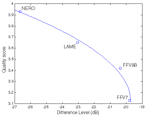
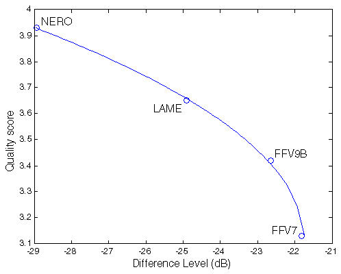
Figure 18. Best quadratic fit between Df measurements and true quality scores with native audio material (a) and the random mix (b).
Below are Df vs. QS scatter plots for all 74 native samples encoded with separate codecs. The first plot corresponds to Fig.18(a). The relationship between Df and QS - less obvious, though - can be seen not only for different codecs but also for different samples encoded with a single codec.
Figure 19. Difference Level vs. Quality score scatter plots for 74 native samples.
Case #2. Public multiformat listening test (July 2014) (33 listeners)
2016 Sep 10
Results of this test along with all supplemental materials were published here - http://listening-test.coresv.net/results.htm. The test was performed mostly by listeners from HydrogenAudio forum using 40 sound samples.
Encoders:
Opus 1.1 with opus-tools-0.1.9-win32
AAC iTunes 11.2.2 via qaac 2.41 (CoreAudioToolbox 7.9.8.5)
Ogg Vorbis aoTuV Beta6.03 [20110424]
MP3 LAME 3.99.5
FAAC-1.28-mod from RareWares
Settings:
opusenc --bitrate 96 in.wav out.opus
qaac --cvbr 96 -o out.mp4 in.wav
venc603 -q2.2 in.wav out.ogg
lame -V5 in.wav out.mp3
faac -b 96 in.wav
faac -q 30 in.wav
Samples:
Total 40 samples (5 sets, 8 samples each).
1. True subjective scores.
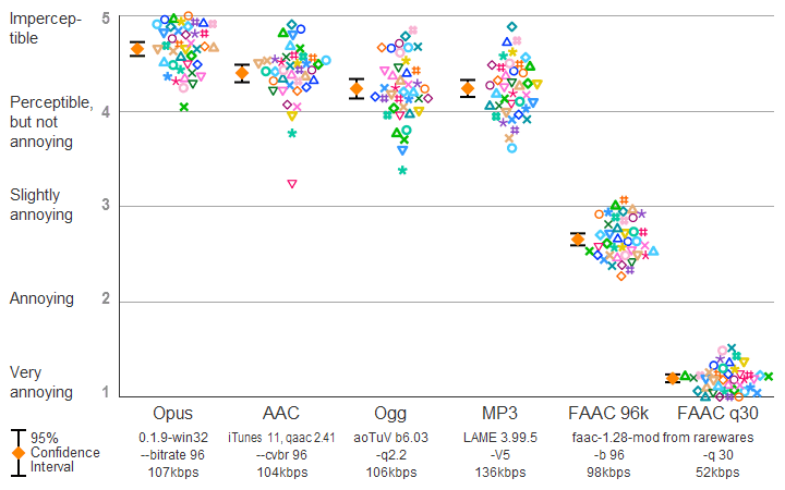 | Figure 201. Results of HA2014 listening test. |
Table 201. Subjective quality scores from the listening test.
AppleAAC  Opus      Ogg       MP3V5     FAAC96k   FAACq30
4.400     4.653     4.235     4.237     2.652     1.194
2. Df measurements.
| Opus |
 |  |
| AAC |
 |  |
| Ogg |
 |  |
| MP3 |
 |  |
| FAAC96k |
 |  |
| FAACq30 |
 |  |
(a)
| (b)
|
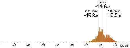
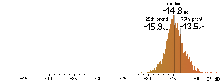
Figure 202. Df measurements with native audio material (a) and the random mix (b).
3. Cluster analysis
Figure 203. Dendrograms of codecs with native audio material (a) and the random mix (b), computed using two clusterization methods: Spearman's rank correlation with average linking (c) and Distance correlation with energy linking (d). Cophenetic correlation shows how good dendrogram represents distances between codecs from distance matrix (Coph <= 1).
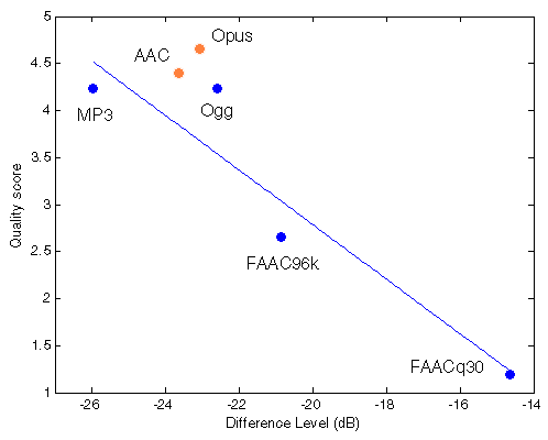
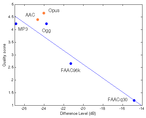
In this listening test all codecs are very different by type of waveform degradation (distances between them are much higher than in Case 1, Fig.17). Nevertheless, in order to estimate the influence of increased distances we will perform usual regression analysis for the group of four codecs: MP3, FAAC96k, Ogg, FAACq30.
Table 202. Distances between codecs with native audio material (left) and the random mix (right) and two measures of distance: Spearman's rank correlation (top) and Distance correlation (bottom). All distances comply with triangle inequality test. The chosen codecs and distances between them are marked with color.
           Opus      AAC       Ogg       MP3       FAAC96k   FAACq30
Opus       000000    0.1569    0.1249    0.1229    0.1769    0.1926
AAC        0.1569    000000    0.1895    0.1574    0.1868    0.2105
Ogg        0.1249    0.1895    000000    0.1128    0.1468    0.1137
MP3        0.1229    0.1574    0.1128    000000    0.0990    0.1595
FAAC96k    0.1769    0.1868    0.1468    0.0990    000000    0.1407
FAACq30 0.1926 0.2105 0.1137 0.1595 0.1407 000000 |
           Opus      AAC       Ogg       MP3       FAAC96k   FAACq30
Opus       000000    0.2104    0.1546    0.1510    0.2391    0.2464
AAC        0.2104    000000    0.1932    0.1827    0.2387    0.2031
Ogg        0.1546    0.1932    000000    0.1180    0.1908    0.1141
MP3        0.1510    0.1827    0.1180    000000    0.1168    0.1472
FAAC96k    0.2391    0.2387    0.1908    0.1168    000000    0.1648
FAACq30 0.2464 0.2031 0.1141 0.1472 0.1648 000000 |
           Opus      AAC       Ogg       MP3       FAAC96k   FAACq30
Opus       000000    0.1835    0.1514    0.1491    0.1975    0.2119
AAC        0.1835    000000    0.2157    0.1823    0.2094    0.2351
Ogg        0.1514    0.2157    000000    0.1365    0.1696    0.1287
MP3        0.1491    0.1823    0.1365    000000    0.1224    0.1861
FAAC96k    0.1975    0.2094    0.1696    0.1224    000000    0.1603
FAACq30 0.2119 0.2351 0.1287 0.1861 0.1603 000000 |
           Opus      AAC       Ogg       MP3       FAAC96k   FAACq30
Opus       000000    0.2415    0.1788    0.1882    0.2677    0.2708
AAC        0.2415    000000    0.2219    0.2172    0.2696    0.2338
Ogg        0.1788    0.2219    000000    0.1478    0.2143    0.1332
MP3        0.1882    0.2172    0.1478    000000    0.1437    0.1744
FAAC96k    0.2677    0.2696    0.2143    0.1437    000000    0.1800
FAACq30 0.2708 0.2338 0.1332 0.1744 0.1800 000000 |
Table 203. Average and Max distances within codecs with native audio material (left) and the random mix (right) and two measures of distance: Spearman's rank correlation (top) and Distance correlation (bottom).
| | Native sound samples | The random mix |
| Average / Max
Spearman's correlation distances
| 0.1288 / 0.1595 | 0.14195 / 0.1908 |
Average / Max
Distance correlation distances | 0.1506 / 0.1861 | 0.16556 / 0.2143 |
4. Regression analysis.
Table 204. True and predicted quality scores with native audio material (a) and the random mix (b).
             MP3       Ogg       FAAC96k   FAACq30   RMSEr

True QS      4.2370    4.2350    2.6520    1.1940
Computed QS  4.5192    3.5343    3.0328    1.2318
Error 6.6602% -16.5466% 14.3580% 3.1642% 0.4234 |
              MP3      Ogg       FAAC96k   FAACq30   RMSEr

True QS      4.2370    4.2350    2.6520    1.1940
Computed QS  4.5012    3.6501    2.9690    1.1976
Error 6.2355% -13.8106% 11.9549% 0.3047% 0.3579 |
| (a) | (b) |
 |  |
(a)
| (b)
|
Figure 204. Best fit (linear) between Df measurements and true quality scores with native audio material (a) and the random mix (b). Codecs not used for computing approximation curves are red.
The errors are expectedly higher. Below are Df vs. QS scatter plots for all 40 native samples.
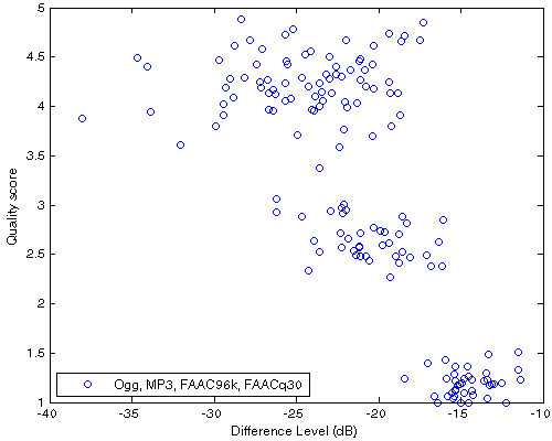 | Figure 205. Df vs. QS scatter plot for 40 native samples encoded with Ogg, MP3, FAAC96k, FAACq30. This is detailed view of averaged quality scores from Fig.204(a) |
Figure 206. Difference Level vs. Quality score scatter plots for 40 native samples.
Case #3. Public AAC Listening Test @ 96 kbps (July 2011)
2016 Sep 20
Results of this test are published here - http://listening-tests.hydrogenaud.io/igorc/aac-96-a/results.html. The test was performed at HydrogenAudio forum by 25 listeners.
Encoders and settings:
- Nero 1.5.4
-q 0.345 - QuickTime 7.6.9, True VBR, via qtaacenc 20101119
--tvbr 46 --highest --samplerate keep - QuickTime 7.6.9, Constrained VBR, via qtaacenc 20101119
--cvbr 96 --highest --samplerate keep - Fraunhofer IIS, via Winamp 5.62
VBR 3 - Coding Technologies, via Winamp 5.61
CBR 100 kbps (.ini file edit to get 100kbps) - ffmpeg's AAC (Lavf53.5.0) @ 96 kbps, Low Anchor
-acodec aac -ab 96k -strict experimental
During the listening test low anchor test files were encoded with ffmpeg build that is no longer in repository. For this research the nearest build was used - ffmpeg-0.8-win64-static (Lavf53.4.0) - which gives difference in third digit after the decimal point in Df measurements. Decoder - Foobar2000 v1.3.11 (32 bit output).
Samples: 20 - https://hydrogenaud.io/index.php/topic,89208.msg763168.html#msg763168
1. True subjective scores.
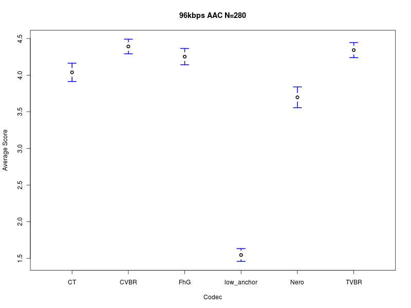 | Figure 301. Results of HA2011 listening test. |
Table 301. Subjective quality scores from the listening test.
Nero      CVBR      TVBR       FhG        CT    low_anchor
3.698     4.391     4.342     4.253     4.039     1.545
2. Df measurements.
 |
Nero |  |
 |
CVBR
|  |
 |
TVBR |  |
 |
FhG |  |
 |
CT |  |
 |
ffmpeg
(anchor) |  |
| (a) | | (b) |
Figure 302. Df measurements with native audio material (a) and the random mix (b).
3. Cluster analysis
Figure 303. Dendrograms of codecs with native audio material (a) and the random mix (b), computed using two clusterization methods: Spearman's rank correlation with average linking (c) and Distance correlation with energy linking (d). Cophenetic correlation (Coph <= 1) shows how good dendrogram represents distances between codecs from distance matrix.
According to above clusterization only three codecs (FhG, Nero, CT) have similar nature of waveform degradation which is insufficient for our regression analysis, so we will use four codecs: FhG, Nero, CT and ffmpeg (anchor); they form the next cluster (with higher within distances though). Tables with distances can be found in c3_mesurements.txt.
Table 302. Average and Max distances within chosen codecs with native audio material (left) and the random mix (right) and two measures of distance: Spearman's rank correlation (top) and Distance correlation (bottom).
                                     Native samples       The random mix
Average / Max
Spearman's correlation distance      0.0780 / 0.1511     0.0855 / 0.1513

Average / Max
Distance correlation distance        0.0955 / 0.1784     0.0991 / 0.1637
4. Regression analysis.
Table 303. True and computed quality scores with native audio material (a) and the random mix (b).
              FhG        CT       Nero     anchor   RMSEr

True QS      4.2530    4.0390    3.6980    1.5450
Computed QS  4.3546    3.4044    4.0420    1.7341
Error +2.39% -15.71% +9.30% +12.24% 0.3766 |
              FhG        CT       Nero     anchor   RMSEr

True QS      4.2530    4.0390    3.6980    1.5450
Computed QS  4.3858    3.3481    4.0267    1.7743
Error +3.12% -17.11% +8.89% +14.84% 0.4048 |
| (a) | (b) |
 |  |
(a)
| (b)
|
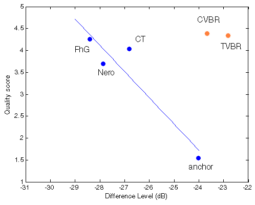
Figure 304. Best fit between Df measurements and true quality scores with native audio material (a) and the random mix (b); in both cases best fit is achieved with linear approximation.
NB! Here we have the first disturbing surprise - loss of monotony of Df/QS dependency for two codecs (Nero, CT); both codecs have very similar nature of waveform degradation but lower Df values correspond to lower quality scores [should be investigated further].
Below are Df vs. QS scatter plots for all 20 native samples.
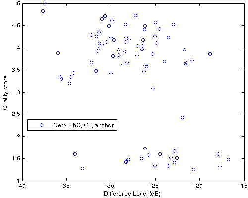 | Figure 305. Df vs. QS scatter plot for 20 native samples encoded with Nero, FhG, CT, ffmpeg (anchor). This is detailed view of the averaged quality scores from Fig.304(a). |
Figure 306. Difference Level vs. Quality score scatter plots for 20 native samples.
Case #4. Public MP3 Listening Test @ 128 kbps (October 2008)
2016 Oct 7
Results of this test are published here - http://listening-tests.hydrogenaud.io/sebastian/mp3-128-1/results.htm. The test was performed at HydrogenAudio forum by 26-39 listeners.
Encoders and settings:
- LAME 3.98.2
-V5.7 - LAME 3.97
-V5 --vbr-new - iTunes 8.0.1.11 (one core)
112 kbps, VBR, highest quality, joint stereo, smart coding, filter below 10 Hz - Fraunhofer IIS CL encoder v1.5
-br 0 -m 4 -q 1 -vbri -ofl - Helix v5.1 2005.08.09
-X2 -U2 -V60 - l3enc 0.99a (Low Anchor)
-br 128000 -mod 1
Decoders: Foobar2000 v1.3.11 (32 bit output) and mp3surround decoder.
Samples: 14 (listed on the results page). Three samples (Vangelis_Chariots_of_Fire, White_Stripes_Hypnotize, sfbay) were not available at the time of the research and they were guessed from full tracks using info from forum discussions and their resulting bitrates.
1. True subjective scores.
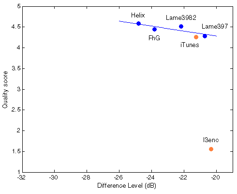
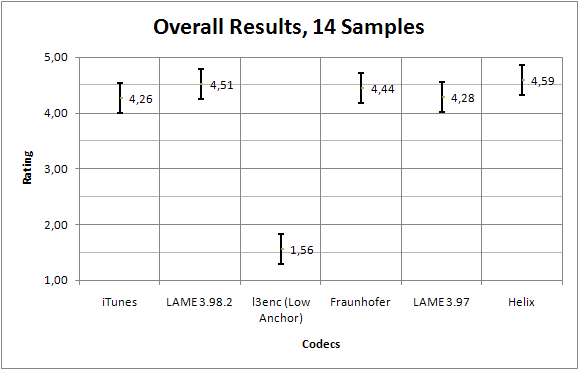 | Figure 401. Results of HA08@128 listening test with mp3 only encoders. |
Table 401. Subjective quality scores from the listening test.
Helix  Lame3982   FhG    Lame397   iTunes   l3enc
4.59     4.51     4.44     4.28     4.26     1.56
2. Df measurements.
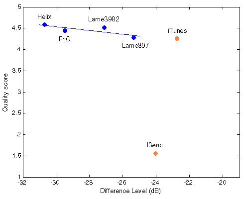
Figure 402. Df measurements with native audio material (a) and the random mix (b).
3. Cluster analysis
Figure 403. Dendrograms of codecs with native audio material (a) and the random mix (b), computed using two clusterization methods: Spearman's rank correlation with average linking (c) and Distance correlation with energy linking (d). Cophenetic correlation shows how good dendrogram represents distances between codecs from distance matrix (Coph <= 1).
According to above clusterization only four MP3 codecs (Lame397, Lame3982, FhG, Helix) have similar nature of waveform degradation. Tables with distances between them can be found in c4_mesurements.txt. Also clusterization with the random mix differs from the one with native samples; probably this is due to small number of samples used in this listening test (14).
Table 402. Average and Max distances within chosen codecs with native audio material and the random mix and two measures of distance: Spearman's rank correlation and Distance correlation.
                                     Native samples       The random mix
Average / Max
Spearman's correlation distance      0.1131 / 0.1730     0.0800 / 0.1196

Average / Max
Distance correlation distance        0.1342 / 0.1918     0.1004 / 0.1494
4. Regression analysis.
Table 403. True and computed quality scores with native audio material (a) and the random mix (b).
              Helix     Lame3982   FhG      Lame397   RMSEr

True QS       4.5900    4.5100    4.4400    4.2800
Computed QS   4.5712    4.4129    4.5108    4.3251
Error -0.41% -2.15% +1.60% +1.05% 0.0649 |
              Helix     Lame3982   FhG      Lame397   RMSEr

True QS       4.2530    4.0390    3.6980    1.5450
Computed QS   4.5674    4.4088    4.5127    4.3310
Error -0.49% -2.24% +1.64% +1.19% 0.0682 |
| (a) | (b) |
Figure 404. Best fit between Df measurements and true quality scores with native audio material (a) and the random mix (b). Codecs not used for computing approximation curves are red.
 |  |
(a)
| (b)
|
Though iTunes MP3 encoder also fits the curve well, this is assumed to be by chance as its type of waveform degradation differs substantially from the others. Indirect prove of the assumption - four chosen codecs preserve their relative positions both with native and random sound material while iTunes changes its position relative to that group.
Scatter plots of individual samples are well-predictable and similar in all cases - clouds around their averages. They are not very informative and will not be provided for the time being.
Case #5. Public Multiformat Listening Test @ ~64 kbps (March 2011)
2017 Apr 23
Results of this test are published here - http://listening-tests.hydrogenaud.io/igorc/results.html. The test was performed at HydrogenAudio forum by 31 listeners (not all listeners tested all samples).
Encoders and settings:
- Nero 1.5.4.0 HE-AAC
-q 0.245 - Ogg Vorbis AoTuV 6.02 Beta
-q 0.1 - Apple QuickTime 7.6.9 HE-AAC
constrained VBR, high quality, 64 kbps - CELT 0.11.2 (March 2011) http://www.celt-codec.org/
complexity 10, VBR 67.5 kbps - iTunes AAC 7.6.9 (Low Anchor)
48 kbps, CBR
Decoders: faad, seltdec, oggdec (the ones used during the test).
Samples: 30 (can be downloaded from the results page above).
1. True subjective scores.
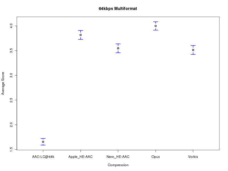 | Figure 501. Results of multiformat HA11@64 listening test (30 samples, 531 results). |
Table 501. Subjective quality scores from the listening test.
Vorbis         Nero_HE-AAC    Apple_HE-AAC   Opus     AAC-LC@48k
3.513          3.547          3.817          3.999    1.656
2. Df measurements.
Figure 502. Df measurements with native audio material (a) and the random mix (b).
3. Cluster analysis
Figure 503. Dendrograms of distances between codecs with native audio material (a) and the random mix (b), computed using two clusterization methods: Spearman's rank correlation with average linking (c) and Distance correlation with energy linking (d). Cophenetic correlation (Coph <= 1) shows how good dendrogram represents distances between codecs from distance matrix.
According to above clusterization there are no any three codecs which are close enough to perform regression analysis. Apple & Nero and Opus & Vorbis are close though. Tables with distances between all codecs can be found in c5_mesurements.txt. Clusterization with the random mix is quite similar to the one with 30 native samples.
Table 502. Average and Max distances within chosen codecs with native audio material and the random mix and two measures of distance: Spearman's rank correlation and Distance correlation.
Not applicable in this case
4. Regression analysis.
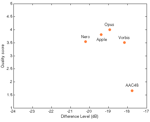
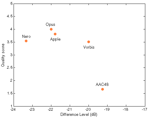
As the regression analysis is not possible in this case Figure 504 shows Df/Score points without fitting curves.
Table 503. True and computed quality scores with native audio material (a) and the random mix (b).
Not applicable in this case
Figure 504. Df/scores scatter plots with native audio material (a) and the random mix (b). All codecs are red as they were not used for computing approximation curves.
 |  |
(a)
| (b)
|
NB! For Apple and Nero our reciprocal monotonity is broken - higher quality scores correspond to higher Df values in both cases (a) and (b).
Analysis of combined HA listening tests' results
2017 Aug 15
To the moment we have results of one personal listening test from Kamedo2 and four listening tests from HA Forum. Earlier HA tests are hardly possible to use for the research as they are poorly documented – codecs and samples used in that tests are hard to find. As a consequence, there is no possibility to compute objective degradation of the stimuli signals. For the above mentioned four HA listening tests we collected all necessary info and will try to analyze their results as a whole (23 codecs in total).
The purpose of such analysis is to find whether these results support our two main working hypotheses:
(1) There is a dependency between degradation of waveform of a stimulus signal and degradation of perceived sound quality of that stimulus signal.
(2) This dependency is more pronounced when type/nature of degradation is similar for tested items.
Note #1.We measure degradation of waveforms with Difference level (Df, dB), perceived sound quality – with Quality scores (Qs) from listening tests and similarity of degradation – with Spareman's distance between sequences of Df values. Each Df sequence represents piece-wise (400ms) degradation of a stimulus signal and can be considered as a degradation signature of a codec. So, similarity of degradation is similarity between degradation signatures.
Note #2. Despite common procedure of conducting HA listening tests there are serious differences between them. First, different sound samples and number of them were used during that tests. Second, different listening subjects and number of them participated in the tests (the number of listeners is also varied for different sound samples). These are two main sources of variance for results of our combined analysis.
Note #3. To keep this analysis simple and easy-to-interpret we will use linear approximation of Qs = f(Df) dependency, thus allowing additional – the third - source of results' variance. In general case a 2nd order curve provides better approximation in least square sense.
Scatter plot of 23 codecs tested during the four HA listening tests is in Fig.HA01.
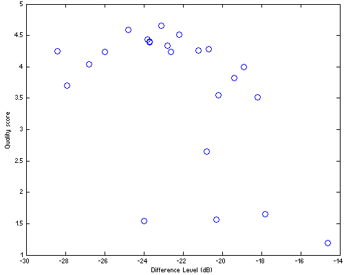 | Figure HA01. Results of four HA listening tests. Number of codecs tested = 23. The codecs are in Df/Qs space, where Qs stands for Quality score and Df – Difference Level (dB) indicates overall waveform degradation of corresponding sound samples (native) used during the test. |
Standard practice of testing a dependency is to measure correlation between variables in question (see Note #3). For our 23 points data set correlation coefficient is 0.52. Bootstrapping this coefficient with n=100000 we get estimation of its 95% confidence interval: [-0.78, -0.11]. Fig.HA02 shows distribution of the bootstrapped values. For comparison the figure also shows distribution of correlation coefficient computed using random sampling with replacement of Df values from our data set.

Figure HA02. Distribution of bootstrapped correlation coefficient. The left histogram is computed using (Df,Qs) values from 23-codec data set; the right histogram is computed using Qs values from 23-codec data set and Df values are randomly sampled with replacement from the data set.
Taking into account serious inconsistency of our 23-codec data set (see Note #2), the overlap of two confidence intervals [-0.42, -0.11] doesn't look so dramatic. The supposed dependency between Df and Qs is quite obvious in the figure.
During our previous separate analyses of HA listening tests (cases 2-5) all participated codecs were used to encode-decode the same Random Mix (in addition to native sound samples). Thus we can measure similarities (distances) between all 23 codecs (see Note #1). Fig.HA03 shows this in the form of dendrogram.
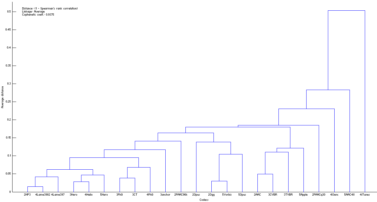 | Figure HA03. Dendrogram of distances between the codecs. It shows similarity of the codecs according to the way they degrade the initial waveform of The Random Mix (click the figure to enlarge). |
Now we can divide our 23-codec data set into n-codec subsets and compute for each subset average distance between codecs and RMS error of their linear approximation. Resulting scatter plots of the subsets for n=4|5|6 are on Fig.HA04.
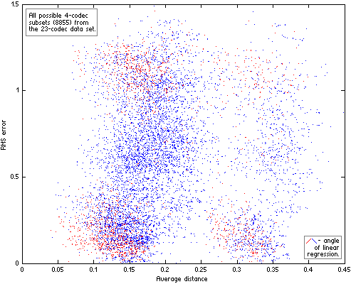 | 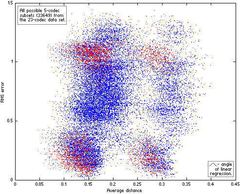 |
| Figure HA04. All possible n-codec subsets of the 23-codec data set. For each subset the two parameters were computed – similarity between codecs in subset (Average distance) and RMS error of their linear approximation. The subsets with “wrong” angle of their linear approximation (quality increases with increase of Df levels) are red. | 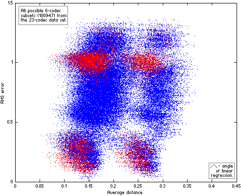 |
Computing distances between codecs with The Random Mix, not the native sound material used in the listening tests, additionally increases variance of RMS errors on the scatter plots (the fourth source of variance). As a result the plots look messy. But even on such imperfect plots the positive trend is quite discernible while “wrong” approximations (in red) are substantially less in quantity and drop out of the trend. In other words, even such inconsistent data support our second hypothesis – the better similarity between codecs, the lower errors of their fit to Df/Qs curve (linear in this particular case). Exactly this relationship between similarity of waveform degradations and goodness of fit of Df and Qs values to some psychometric curve has the highest practical value as it helps to determine in what cases listening tests can be safely substituted with objective measurements. Unfortunately the data from HA listening tests are suitable only for qualitative estimation of that dependency. Quantitative estimations are possible only with more consistent data, which can be obtained from properly organized listening test with multiple testing items or series of proper tests with the same panel of listening experts and the same set of sound samples.
to be continued ...