Part 1
Draft. 2014 Sep 10. Live research.
From the early days of SoundExpert the objective audio parameter – signal difference level (Df) – was actively used for audio research within the project. This simple parameter shows difference between a reference (input) waveform and a processed (output) one. It is defined as follows:
Df [%] = (1 - |p|) * 100 or Df [dB] = 10 * Log10(1 - |p|), where p is correlation coefficient.
When signals' waveforms are identical, Df = -Infinity [dB]; when the forms are completely different, Df = 0 [dB]; levels and DC offsets of both signals do not affect difference level. The main beauty of the parameter is that it can be used with signals of any shape, both synthetic (sine, white noise, …) and real-life (music, voice, ...). So, in order to evaluate some device under test you can feed it with various signals and measure degradation of those signals with one and the same parameter. For sinusoidal signals Df[dB] approximately equals to (THD – 3.01).
Df can be computed for any signal of any duration, for a whole signal or for any part of it. Usual time blocks of 50+ ms (Tb) are very suitable for Df calculation. To visualize Df values throughout a signal they can be color coded, showing distortion of different signal sections. Example of such diffrogram is shown in Fig.1.
 | Fig.1. Diffrogram of glockenspiel sample played back by iPhone 5s. Each 1 pixel bar represents 50 ms (Tb) of the signal. Green areas correspond to lower distortion (lower Df values, closer to -Inf [dB]), red ones correspond to higher degradation of initial waveform of the sample. Mean Df of all time blocks is -27.7 dB.
Tb = 50 ms
Df = -27.7 dB |
Diffrogram becomes more revealing when combined with spectrogram. As color is already used for Df visualization, amplitude of spectral components can be coded with lightness/darkness of color. Fig.2 shows such enhanced diffrogram from the previous example.
 | Fig.2. Diffrogram from Fig.1 combined with spectrogram. Hue of color represents difference level, lightness/darkness of color represents amplitude of frequency components.
Tb = 50 ms
Df = -27.7 dB |
Color map of (difference level, amplitude) space is shown in Fig.3.
Below are some trivial examples with sinusoidal signals which help to understand diffrograms better and which show the accuracy of Df computation. First set of examples are sine signals (1 kHz, 10 sec) of three different levels (-3dBFS, -9dBFS, -27dBFS) quantized (without dithering) from 32bit(float) to 24bit and 16bit:
 | REF: sine 1kHz, -3dBFS, 32bit
OUT: sine 1kHz, -3dBFS, 24 bit
Tb = 100 ms
Df = -144.7 dB |  | REF: sine 1kHz, -9dBFS, 32 bit
OUT: sine 1kHz, -9dBFS, 24 bit
Tb = 100 ms
Df = -140.4 dB |  | REF: sine 1kHz, -27dBFS, 32 bit
OUT: sine 1kHz, -27dBFS, 24 bit
Tb = 100 ms
Df = -122.3 dB |
| |
 | REF: sine 1kHz, -3dBFS, 32 bit
OUT: sine 1kHz, -3dBFS, 16 bit
Tb = 100 ms
Df = -97.9 dB |  | REF: sine 1kHz, -9dBFS, 32 bit
OUT: sine 1kHz, -9dBFS, 16 bit
Tb = 100 ms
Df = -92.2 dB |  | REF: sine 1kHz, -27dBFS, 32 bit
OUT: sine 1kHz, -27dBFS, 16 bit
Tb = 100 ms
Df = -73.8 dB |
Fig.4. Diffrograms of sinusoidal signals of different levels, quantized from 32bit(float) to 24bit and 16bit. Quantization errors are higher at lower levels. |
Signals of lower levels are subject to higher levels of degradation (quantization errors) and this is indicated by color. Non-uniform color on -3dBFS/24bit diffrogram reflects computational errors of extremely low Df values. Thus, difference level -140 dB could be considered as maximum accuracy of Df computation using current algorithm.
Accuracy of Df measurement is affected not only by computational error. Even slightest time misalignment of input and output signals makes calculation of Df impossible. While digital processing of signals is usually time accurate, conversion from digital to analog and vice versa is not. All analog signals must be precisely time warped before computing of Df. The next set of examples shows accuracy of this part of measurement procedure. Once again, sinusoidal signals are very appropriate for the case as they can be easily generated in digital form with any parameters and the shapes of all sine waves are perfectly identical by definition. In the following set of examples Df values were computed with sine signals of slightly deviated frequencies. As our time warping procedure is sensitive to sampling rate of a signal, Df values were computed for five different frequencies (1, 5, 10, 15, 20 [kHz]) and four sampling rates (44101, 96002, 192004, 384009 [Hz]).
 | REF: sine 1k(44100)
OUT: sine 1k(44101)
Tb = 100 ms
Df = -143.5 dB |  | REF: sine 1k(44100)
OUT: sine 1k(96002)
Tb = 100 ms
Df = -145.5 dB |  | REF: sine 1k(44100)
OUT: sine 1k(192004)
Tb = 100 ms
Df = -143.6 dB | | |
| |
 | REF: sine 5k(44100)
OUT: sine 5k(44101)
Tb = 100 ms
Df = -82.7 dB |  | REF: sine 5k(44100)
OUT: sine 5k(96002)
Tb = 100 ms
Df = -102.2 dB |  | REF: sine 5k(44100)
OUT: sine 5k(192004)
Tb = 100 ms
Df = -126.5 dB | | |
| |
 | REF: sine 10k(44100)
OUT: sine 10k(44101)
Tb = 100 ms
Df = -51.4 dB |  | REF: sine 10k(44100)
OUT: sine 10k(96002)
Tb = 100 ms
Df = -76.6 dB |  | REF: sine 10k(44100)
OUT: sine 10k(192004)
Tb = 100 ms
Df = -101.5 dB | | |
| |
 | REF: sine 15k(44100)
OUT: sine 15k(44101)
Tb = 100 ms
Df = -30.9 dB |  | REF: sine 15k(44100)
OUT: sine 15k(96002)
Tb = 100 ms
Df = -61.0 dB |  | REF: sine 15k(44100)
OUT: sine 15k(192004)
Tb = 100 ms
Df = -87.1 dB | | |
| |
 | REF: sine 20k(44100)
OUT: sine 20k(44101)
Tb = 100 ms
Df = -13.9 dB |  | REF: sine 20k(44100)
OUT: sine 20k(96002)
Tb = 100 ms
Df = -49.1 dB |  | REF: sine 20k(44100)
OUT: sine 20k(192004)
Tb = 100 ms
Df = -76.6 dB |  | REF: sine 20k(44100)
OUT: sine 20k(384009)
Tb = 100 ms
Df = -102.2 dB |
Fig.5. Diffrogramms of sinusoidal signals (-3dBFS, 10sec) of slightly deviated frequencies. They show accuracy of time warping algorithm at different sampling rates. |
As all sine waveforms are identical, the above diffrograms show accuracy of time warping procedure. According to the figure max. accuracy of time warping of frequencies around 20k at 384k sampling rate is -102 dB. So, calculation of difference levels below -100 dB for full bandwidth analog signals (which always require time warping) should be done at 10x sampling rate or higher.
Now we are ready to compute diffrograms for some real life audio signals. Figure 6 shows diffrograms of glockenspiel sample quantized from 32bit(float) to 24bit and 16bit. Figure 7 shows this sample up-sampled from 44100 to 96000 Hz in Adobe Audition and in foobar2000; both using max. quality settings.
 | REF: GLK 32bit (44100)
OUT: GLK 24bit (44100)
Tb = 50 ms
Df = -114.8 dB |  | REF: GLK 32bit (44100)
OUT: GLK 32bit (96000, AA)
Tb = 50 ms
Df = -84.5 dB |
| |
 | REF: GLK 32bit (44100)
OUT: GLK 16bit (44100)
Tb = 50 ms
Df = -67.5 dB |  | REF: GLK 32bit (44100)
OUT: GLK 32bit (96000, fb)
Tb = 50 ms
Df = -74.3 dB |
Fig.6. Diffrograms of glockenspiel sample quantized from 32bit(float)
to 24bit and 16bit. |
Fig.7. Diffrograms of glockenspiel sample up-sampled from 44100Hz to 96000Hz
in Adobe Audition CS6 (AA) and foobar2000 v1.3.3 (fb). |
Even taking into account inaccuracy of time warping of high frequencies at 96000 sampling rate we can safely conclude from fig.7 that up-sampling in Audition CS6 preserves initial (reference) waveform better than upsampling in foobar2000 - mean Df values and colors are quite indicative.
The next set of diffrograms could be considered as real-life application of this new audio metric. We'll use it for evaluation of three portable devices:
- FiiO E17 - USB DAC headphone amplifier
- iPhone 5s - smartphone
- iPhone 6 - smartphone
- iriver E100 - multimedia player
Sinusoidal signal (1kHz, -15dBFS, 44100Hz, 16bit, 20sec), white noise (-15dBFS, 44100Hz, 16bit, 20sec) and nine SE test samples (44100Hz, 16bit) were played back on these devices (left channel only) at matched levels and recorded from headphone outputs (loaded with 33Ohm resistors) with MicroTrack at 96k/24bit.
Below are diffrograms of these three portable devices and the above signals:
 | REF: sine 1k, 44100Hz, 16bit
OUT: FiiO E17, 96000Hz, 24bit
Tb = 100 ms
Df = -72.3 dB |  | REF: white noise, 44100Hz, 16bit
OUT: FiiO E17, 96000Hz, 24bit
Tb = 100 ms
Df = -29.5 dB |
| |
 | REF: sine 1k, 44100Hz, 16bit
OUT: iPhone 5s, 96000Hz, 24bit
Tb = 100 ms
Df = -70.5 dB |  | REF: white noise, 44100Hz, 16bit
OUT: iPhone 5s, 96000Hz, 24bit
Tb = 100 ms
Df = -4.5 dB |
| |
 | REF: sine 1k, 44100Hz, 16bit
OUT: iPhone 6, 96000Hz, 24bit
Tb = 100 ms
Df = -70.6 dB |  | REF: white noise, 44100Hz, 16bit
OUT: iPhone 6, 96000Hz, 24bit
Tb = 100 ms
Df = -4.6 dB |
| |
 | REF: sine 1k, 44100Hz, 16bit
OUT: iriver E100, 96000Hz, 24bit
Tb = 100 ms
Df = -70.6 dB |  | REF: white noise, 44100Hz, 16bit
OUT: iriver E100, 96000Hz, 24bit
Tb = 100 ms
Df = -18.0 dB |
Fig.8. Diffrograms of FiiO E17, iPhone 5s, iPhone 6 and iriver E100
with sinusoidal signal. |
Fig.9. Diffrograms of FiiO E17, iPhone 5s, iPhone 6 and iriver E100
with white noise signal. |
While all three devices show almost similar performance with sine signal, white noise reveals significant distinctions in its reproduction. These distinctions are also evident on diffrograms of these devices with nine SE samples:

REF: SE samples, 44100Hz, 16bit; OUT: FiiO E17, 96000Hz, 24bit; Tb = 100 ms; Df = -26.6 dB |
| |

REF: SE samples, 44100Hz, 16bit; OUT: iPhone 5s, 96000Hz, 24bit; Tb = 100 ms; Df = -24.6 dB |
| |

REF: SE samples, 44100Hz, 16bit; OUT: iPhone 6, 96000Hz, 24bit; Tb = 100 ms; Df = -24.4 dB |
| |

REF: SE samples, 44100Hz, 16bit; OUT: iriver E100, 96000Hz, 24bit; Tb = 100 ms; Df = -16.7 dB |
| |
| Fig.10. Diffrograms of FiiO E17, iPhone 5s, iPhone 6 and iriver E100 with nine SE samples. |
At this point we are not trying to explain distinctions on these diffrograms and their impact on perceived audio quality of the devices. We can just establish the fact that various signals are transferred through these devices with various precision. In order to show that the relationship between objectively measured signal difference level and subjective perception of sound quality is not trivial (as well as for the purpose of some soft scientific trolling), here is a set of diffrograms of Lame (3.99.5) mp3 encoder at different quality settings (-V) with the nine SE samples:

REF: SE samples, 44100Hz, 16bit; OUT: Lame -b 320, 44100Hz, 32bit; Tb = 100 ms; Df = -48.3 dB |
| |

REF: SE samples, 44100Hz, 16bit; OUT: Lame -V0, 44100Hz, 32bit; Tb = 100 ms; Df = -40.8 dB |
| |

REF: SE samples, 44100Hz, 16bit; OUT: Lame -V1, 44100Hz, 32bit; Tb = 100 ms; Df = -38.3 dB |
| |

REF: SE samples, 44100Hz, 16bit; OUT: Lame -V2, 44100Hz, 32bit; Tb = 100 ms; Df = -35.9 dB |
| |

REF: SE samples, 44100Hz, 16bit; OUT: Lame -V3, 44100Hz, 32bit; Tb = 100 ms; Df = -34.5 dB |
| |

REF: SE samples, 44100Hz, 16bit; OUT: Lame -V4, 44100Hz, 32bit; Tb = 100 ms; Df = -32.4 dB |
| |

REF: SE samples, 44100Hz, 16bit; OUT: Lame -V5, 44100Hz, 32bit; Tb = 100 ms; Df = -29.1 dB |
| |

REF: SE samples, 44100Hz, 16bit; OUT: Lame -V6, 44100Hz, 32bit; Tb = 100 ms; Df = -26.4 dB |
| |

REF: SE samples, 44100Hz, 16bit; OUT: Lame -V7, 32000Hz, 32bit; Tb = 100 ms; Df = -25.4 dB |
| |

REF: SE samples, 44100Hz, 16bit; OUT: Lame -V8, 24000Hz, 32bit; Tb = 100 ms; Df = -26.9 dB |
| |

REF: SE samples, 44100Hz, 16bit; OUT: Lame -V9, 22050Hz, 32bit; Tb = 100 ms; Df = -24.5 dB |
Fig.11. Diffrograms of Lame 3.99.5 at different quality settings with nine SE samples. |
Obviously, degradation of initial waveform in iPhone 6 (Df = -24.4dB) and in Lame -V9 (Df = -24.5dB) has different consequences for perceived audio quality. So, comparison of Df values should be done with great care.
Nevertheless, Df values in the form of diffrogram could give valuable insights into features of a signal processing being investigated. For this purpose short time blocks (Tb = 50ms) are more appropriate. Equally, diffrogram can be computed with extensive and greatly varied audio material and then resulting Df values can be analyzed with statistical methods. In this case 400ms-3sec time blocks are more helpful. Exactly thanks to possibility of using various signals for computing difference level, the parameter and diffrogram have high research potential. To be continued ...
Part 2
Draft. 2015 Jan 25. Live research.
Before we continue some changes should be noted:
- standard logarithmic scale of frequencies is used now for spectrogram (see Fig.12) instead of square-law scale used in Part 1
- Median looks like a better estimator of central tendency for Df values, so it is used now instead of Mean
- instead of Time block the standard term Time window is used for computing a single Df value (Tw = Tb)
|  | Figure 12. “New” logarithmic frequency scale for spectrogram. The old one is in Fig.2.
Tw = 50 ms
Df(median) = -29.3 dB |
Difrorgams below show distortion of some standard test signals (30sec, -10dBFS RMS) which have been transferred through the device under test – iBasso DX50 audio player (mono(L+R), resistive 33 Ohm load).
 | Figure 13. Diffrogram of DX50 with sinusoidal signal 1kHz
REF: sine 1kHz, 44100Hz, 16bit
OUT: iBasso DX50, 96000Hz, 24bit
WarpFrame = 30s
Tw = 100ms
Df(min)= -79.5 dB, Df(median)= -79.1 dB |
 | Figure 14. Diffrogram of DX50 with sinusoidal signal 12.5kHz. Slow change of Df values reflect instability of DX50 internal clock. Testing sine signal of higher frequency better reveals oscillation, which is not noticeable at 1kHz.
REF: sine 12.5kHz, 44100Hz, 16bit
OUT: iBasso DX50, 96000Hz, 24bit
WarpFrame = 30 s
Tw = 100 ms
Df(min)= -78.9 dB, Df(median)= -64.8 dB |
 | Figure 14.1. Diffrogram of DX50 with sinusoidal signal 12.5kHz as in Fig.14 but with smaller time frame for warp processing (100ms instead of 30s). Oscillation of sampling frequency is not noticeable in this case; accuracy of reproduction of sine 12.5k is only slightly worse than of sine 1k from Fig.13.
REF: sine 12.5kHz, 44100Hz, 16bit
OUT: iBasso DX50, 96000Hz, 24bit
WarpFrame = 100 ms
Tw = 100 ms
Df(min)= -79.4 dB, Df(median)= -78.8 dB |
 | Figure 15. Diffrogram of DX50 with DFD signal: 12.5 kHz mean, 80 Hz difference (12460 Hz + 12540 Hz). For elimination of sampling frequency oscillation warping time frame is also set to 100ms. Lower Df values in comparison with Fig.14.1 reveal presence of inter-modulation distortion (IMD).
REF: DFD 12.5kHz, 44100Hz, 16bit
OUT: iBasso DX50, 96000Hz, 24bit
WarpFrame = 100 ms
Tw = 100 ms
Df(min)= -75.3 dB, Df(median)= -75.0 dB |
 | Figure 16. Diffrogram of DX50 with MOD-SMPTE 4-to-1 signal: 60 Hz + 7 kHz, 4:1. Substantially lower Df values are caused by phase inaccurate reproduction of different frequencies in iBasso DX50. This test signal is highly affected by parameters of time warping and is not suitable for IMD assessment within Df metric.
REF: MOD-SMPTE 4-to-1, 60 Hz + 7 kHz, 44100Hz, 16bit
OUT: iBasso DX50, 96000Hz, 24bit
WarpFrame = 100 ms
Tw = 100 ms
Df(min)= -47.4 dB, Df(median)= -47.4 dB |
 | Figure 17. Diffrogram of DX50 with Sweep tone 20Hz-20kHz (linear). Df values increase slightly with frequency (“greener” right end) visually indicating that higher frequencies are reproduced with lower accuracy. This test signal is highly affected by parameters of time warping and should be used with caution.
REF: sweep 20-20kHz, 44100Hz, 16bit
OUT: iBasso DX50, 96000Hz, 24bit
WarpFrame = 200 ms
Tw = 100 ms
Df(min)= -79.5 dB, Df(median)= -78.4 dB |
 | Figure 18. Diffrogram of DX50 with square wave 1kHz. This wave-form is distorted much higher than the sine wave from Fig.13
REF: square wave 1 kHz, 44100Hz, 16bit
OUT: iBasso DX50, 96000Hz, 24bit
WarpFrame = 100 ms
Tw = 100 ms
Df(min)= -37.4 dB, Df(median)= -37.4 dB |
 | Figure 19. Diffrogram of DX50 with white noise.
REF: white noise, 44100Hz, 16bit
OUT: iBasso DX50, 96000Hz, 24bit
WarpFrame = 100 ms
Tw = 100 ms
Df(min)= -26.6 dB, Df(median)= -25.0 dB |
 | Figure 20. Diffrogram of DX50 with “program simulation noise” (BS EN 50332-1), whose spectral content is representative of music and speech. A good candidate for being a “standard” test signal within Df metric.
REF: pink noise, filtered and dynamically compressed (BS EN 50332-1), 44100Hz, 16bit
OUT: iBasso DX50, 96000Hz, 24bit
WarpFrame = 100 ms
Tw = 100 ms
Df(min)= -22.4 dB, Df(median)= -19.4 dB |
The list of possible test signals is limited only by creativity of researcher. Though not all of them are useful within Df audio metric. Additional research is required.
Each diffrogram provides a set of Df values which can be further analyzed with statistical methods. For example Fig.21 shows diffrogram of iBasso DX50 with nine SE samples and Fig.22 shows histogram of these Df values.

Figure 21. Diffrogram of iBasso DX50 with nine SE samples.
REF: SE samples, 44100Hz, 16bit; OUT: iBasso DX50, 96000Hz, 24bit; Tw = 100 ms; Df(min)= -47.8 dB, Df(median)= -23.2 dB

Figure 22. Histogram of Df values (N=931) from diffrogram in Fig.21.
REF: SE samples, 44100Hz, 16bit; OUT: iBasso DX50, 96000Hz, 24bit; Tw = 100 ms; Df(min)= -47.8 dB, Df(median)= -23.2 dB
As SE samples represent different types of audio material and the number of Df values (N=931) is relatively small the distribution of Df looks pretty random. For big N the distribution becomes “more Gaussian”. For example, using the whole Pink Floyd album “The Dark Side Of The Moon” (Discovery Edition, 2011 Remaster, EMI) as a test signal gives 6440 Df values (Tw=400ms). Diffrogram of the third track “On The Run” is shown in Fig.23.

Figure 23. Diffrogram of iBasso DX50 with “On The Run” track by Pink Floyd.
REF: Pink Floyd, “On The Run”, 3:45, 44100Hz, 16bit; OUT: iBasso DX50, 96000Hz, 24bit; Tw = 400 ms; Df(min)= -25.7 dB, Df(median)= -19.4 dB
Histogram of Df values for iBasso DX50 with the whole album “The Dark Side Of The Moon” (N=6440) is shown in Fig.24. For comparison Fig.25 shows similar histogram for another audio player - iriver E100.

Figure 24. Histogram of Df values for iBasso DX50 with the whole album “The Dark Side Of The Moon” (N=6440).
REF: Pink Floyd, “The Dark Side Of The Moon”, 43:00, 44100Hz, 16bit; OUT: iBasso DX50, 96000Hz, 24bit; Tw = 400 ms; Df(min)= -39.1 dB, Df(median)= -20.1 dB

Figure 25. Histogram of Df values for iriver E100 with the whole album “The Dark Side Of The Moon” (N=6440).
REF: Pink Floyd, “The Dark Side Of The Moon”, 43:00, 44100Hz, 16bit; OUT: iriver E100, 96000Hz, 24bit; Tw = 400 ms; Df(min)= -34.5 dB, Df(median)= -16.8 dB
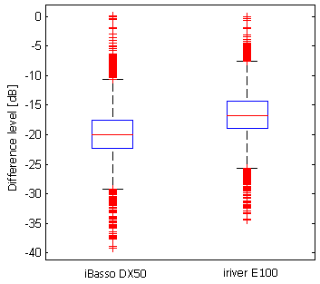
Pretty evident that one player preserves initial waveform better than the other. Comparison of such Df sets can be done with standard boxplots showing median and 25\75 percentiles of data, thus giving estimation of location and spread of Df values (Fig.26).
 | Figure 26. Boxplot of Df values (N=6440) for two audio players. Each Df value estimates similarity of a small portion (400ms) of initial digital waveform with corresponding portion at headphone output of player. The less the value in dB, the better. |
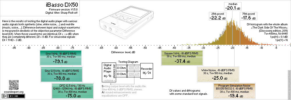
And finally all objective measurements according to this audio metric could be summarized as in Fig.27 showing performance of device under test with various test signals in one simple view.

Figure 27. Results of testing iBasso DX50 digital audio player with various audio signals and single measurement approach based on Difference level parameter.
Diffrogram utility (Matlab)
Matlab code for computing Difference levels and building diffrograms; with examples of usage.
diffrogram_v3.34.zip (9.8kB) - correct phase computation, no readme (soon), help is in the code
diffrogram_v3.33.zip (9.5kB) - more accurate stereo-to-mono conversion, precise freq. scale, no readme (soon), help is in the code
diffrogram_v3.32.zip (8.8kB) - power output added, no readme (soon), help is in the code
diffrogram_v3.31.zip (8.8kB) - bug fix, no readme (soon), help is in the code
diffrogram_v3.3.zip (8.7kB) - no readme (soon), help is in the code
diffrogram_v2.4.zip (12.6M) - calibrated accuracy
diffrogram_v2.3.zip (872k) - usability improvements
diffrogram_v2.2.zip (832k) - first public release